Traffic Analysis Toolbox Volume III: Guidelines for Applying Traffic Microsimulation Modeling Software 2019 Update to the 2004 Version

Chapter 5. Model Calibration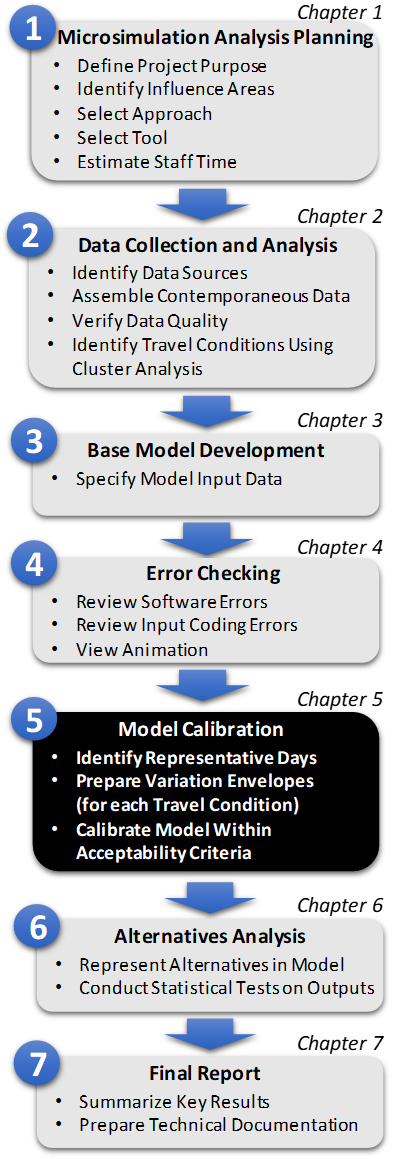

Upon completion of the error-checking task, the analyst has a working model of the transportation system. However, without calibration, the analyst has no assurance that the model will function as an accurate predictor of transportation system performance in alternatives analysis.

This is Step 5 in the Microsimulation Analytical Process (Figure 9). Calibration is the adjustment of model parameters to improve the model's ability to reproduce time-dynamic system performance observed under specific travel conditions. Note that variation in transportation system performance is primarily determined by external variations in travel conditions (e.g., variations in day-to-day travel demand, incident patterns, and weather conditions). Driver behavior (e.g., following distance, gap acceptance, and target maximum speed) and other model parameters are calibrated in each travel condition to create time-dynamic congestion patterns consistent with observed data.

Calibration is necessary because no single model can be expected to be equally accurate for all possible traffic conditions. Even the most detailed microsimulation model still contains only a portion of all of the variables that affect real-world traffic conditions. Since no single model can include the whole universe of variables, every model should be adapted to local conditions.

Every microsimulation software program comes with a set of user-adjustable parameters for the purpose of calibrating the model to local conditions. Therefore, the objective of calibration is to find the set of parameter values for the model that best reproduces observed measures of system performance.

For the convenience of the analyst, the software developers provide suggested default values for the model parameters. These default parameters do not represent a calibrated model. The analyst should always perform model calibration and review the calibration criteria to ensure that the model accurately reproduces system performance by travel condition.

Overview of the Calibration Process

As shown in Figure 9, the calibration process has three steps:

1. Identify representative days. In this step, the analyst takes the data from the travel conditions identified using cluster analysis or other statistical methods (Chapter 2) and prepares them to support calibration. A key element of this preparation is the identification of one representative day for each travel condition.
2. Prepare variation envelopes. In this step, the analyst prepares the simulation inputs to model each representative day. For each representative day, the analyst creates a time-dynamic envelope consistent with variation in observed field data for all days in the cluster representing the travel condition. This envelope creates a data-driven calibration target for the calibration of an individual model variant consistent with each travel condition.
3. Calibrate model variants within acceptability criteria. The analyst then iteratively adjusts specific software parameters within a model variant until key performances measures derived from simulation outputs are acceptably close to the target variation envelope. Calibration of each model variant is complete when the simulation outputs meet four acceptability criteria.

The calibration process is applied to a single model run for each travel condition or cluster identified in Chapter 2. The analyst does not need to calibrate multiple model runs generated by varying the random number seeds. Variation demonstrated by varying random number seeds in microsimulation tools show differences in driver behaviors (e.g., gap acceptance, lane changing), and vehicles entering the system. These variations are markedly low compared to variation due to changes in travel condition attributes (e.g., demand, weather), which are not represented stochastically in microsimulation tools. If significant variations are seen between runs by changing the random number seeds, a possible reason might be errors in coding or gridlock conditions resulting from vehicles entering into unresolved contention in simulation (e.g., vehicles attempting conflicting parallel lane changes). An analyst should investigate if the network has been coded correctly and is operating realistically or if the model is unstable. The results from an unstable model run should not be used for calibration or alternatives analysis.

In the remainder of this section, we describe in detail each of the three steps, using the Alligator City hypothetical simulation study as an example.

Identify Representative Days

In this step, we prepare and assemble observed data related to our key performance measures and network bottlenecks. Observed data are organized around the travel conditions identified in Chapter 2. Travel conditions and performance measures should be identified in the Analysis Plan. Depending on an assessment of quality of data, there may be a need to adjust the selection of specific measures prior to calibration. Critical locations (bottlenecks) are identified for each travel condition, plus a super set of all bottlenecks maintained comprising all travel conditions.

It is important to focus calibration on a single observed day, since that day can be characterized in a microsimulation model with specific incident locations, travel times, and other performance data. Attempting to calibrate a model to a synthetic day created by the averaging together of multiple days is not recommended. Synthetic days based on averages create unrealistically smooth time dynamic performance measures like travel time and bottleneck throughput, creating targets that may be difficult for any model variant to replicate. For example, if one day has a major incident in one location and is then averaged with a day with no incident, then the result is the merging of two broadly dissimilar days. The analyst should now attempt to somehow induce a more minor incident in that location to produce a moderated congestion pattern. In fact, the resulting synthetic measures of system performance may not even be consistent with logically consistent traffic flow, and may be exceptionally difficult to reproduce in a valid modern microsimulation. In this case, the analyst wastes resources calibrating to a condition that never existed and will likely never exist.

For each travel condition, the analyst seeks to identify a single representative day. The representative day is used to typify system performance dynamics associated with the collection of days encompassing a single travel condition. More precisely, the representative day and has observed time-variant performance measures closest to mean time-dependent observed measures considering all days in the travel condition.

In order to identify the representative day, time-variant data related to the key performance measures are analyzed. For every day used in the analysis across all travel conditions, the analyst prepares a time-variant (15-minute profile) of the key measure. Multiple locations and routes may be required to characterize system performance. For example, in corridor networks with alternatives, travel time and speed measures may be needed on multiple routes. Likewise, there may be multiple bottleneck locations within the system. To identify a representative day:

1. For a particular key measure, establish necessary routes and locations.

   Let \(M\) be the set of measures, considered over \(J\) the set of routes and locations.

   Let \(N_{\text{cluster}}\) be the number of days in cluster.

   Let \(m_{i,j}(t)\) be the value of the measure on day \(i\) in time interval \(t\) at location or route \(j\)

2. For each measure, calculate the average time-variant value for each 15-minute time interval across all days in the travel condition for each location/route:

   \({\overline{m}}_{t,j} = \frac{\sum_{i}^{}{m_{i,j}(t)}}{N_{\text{cluster}}}\ \ \forall m,\ t,\ j\)(5)

3. Calculate the difference between the average value and the value observed on a particular day, expressed as a percentage of the mean value:

   \({\dot{m}}_{i,j}\left( t \right) = \frac{\sqrt{{({\overline{m}}_{t,j} - {\overline{m}}_{i,j(t)})}^{2}}}{{\overline{m}}_{t,j}}\)(6)

4. Find the individual day that minimizes the difference between the individual day and the average values considering all routes, locations, and measures:

   \(i^{*} = \min_{i}\left\lbrack \sum_{m}^{}{\sum_{i}^{}{\sum_{t}^{}{{\dot{m}}_{i,j}(t)}}} \right\rbrack\)(7)

Prepare Variation Envelopes

Select Calibration Performance Measures

An effective calibration requires at least two key performance measures. At least one measure should be related to travel time or speed profiles along one or more key paths in the roadway network. At least one other measure should be related to bottleneck dynamics, e.g., bottleneck throughput or duration. Other calibration measures can also be included that are critical to the purpose and needs of the project or in differentiating alternatives evaluated in the analysis. However, whatever measures are selected, the data required to calculate each measure for the purposes of calibration are required for every day included in the analysis of travel conditions. The ability to meet these data preparation guidelines for calibration should be documented in the accompanying project Methods and Assumptions document.

Travel time or speed measures. Travel times or speed profiles should be associated with paths that traverse the study area and intersect at least one bottleneck location on the representative day. Observed data should be available for these measures and paths at 15-minute (or more frequent) intervals. More than one path may be required to capture the system dynamic, or in corridor analyses, the mainline and one alternative path. An interchange analysis might require only one path.

Bottleneck measures. For every day across all travel conditions, identify the set of bottleneck locations. Bottleneck locations are defined as the set of network locations where transient demand exceeds facility capacity and resultant approach speeds drop below the bottleneck congestion speed threshold.

Data for the calculation of bottleneck measures are best derived from data obtained from at least one near upstream (within 0.5 miles and prior to any major intersection or interchange) or near downstream location for at least one bottleneck associated with the travel condition. Near downstream locations are preferred, prior to the next major intersection or interchange.

Congestion speed threshold: For this threshold, the analyst requires a value lower than approximate speed-at-capacity and closer to speed-at-congestion, that is, a speed that indicates that the bottleneck has reached or exceeded its capacity. As a rule of thumb, a threshold of one third of observed free-flow speed can be used with visual inspection of time-variant speed and flow rates at the bottleneck for the representative day. However, speed at capacity can be more precisely calculated using other data-driven approaches (For example, https://www.academia.edu/11327450/An_automated_statistically-principled_bottleneck_identification_algorithm_ASBIA). The goal of the analyst is selecting a threshold that is lower than speed-at-capacity and can be applied uniformly across all days in the travel condition.

For each bottleneck location, calculate bottleneck onset and duration. Onset and duration are identified at least within a 15-minute time intervals.

Congestion onset: Onset is defined as the 15-minute time period when a location immediately upstream of the bottleneck experiences observed speeds below the congestion speed threshold.

Congestion duration: Total time observed between congestion onset at the bottleneck location and the 15-minute period where average observed speeds exceed the congestion speed threshold.

For bottleneck attributes, it is imperative to focus on a specific observed representative day when conducting calibration. Aggregating bottleneck measures blurs distinctions among bottlenecks and often results in multiple "weak" bottlenecks with inconsistent time-dependent flow rates. These artificial conditions are never observed in a single day, and are difficult for a microsimulation to reproduce.

Onset and duration speed measurements should, if possible, be collected at a near upstream location. If not possible, document these as a deviation in the Methods and Assumptions document. Average mean space speed or mean point speed may be utilized whichever best characterizes the bottleneck performance. For example, a mean space speed may be preferable for a bottleneck upstream from a signalized intersection.

Creating Variation Envelopes

Our goal in calibration is to have the variation of results generated by the simulation fall within the range of variation seen in the observed data. In Chapter 2, we defined travel conditions. From the limited variation resulting from our travel condition analysis, in this step we create a practical range derived from the observed variation to act as a target for model variant calibration.

To create the time-variant Variation Envelope for our simulation results to fall within, we create a statistical region based on the standard deviation and an acceptable range of variation around both the time variant averages and the observed representative day value.

Let c_r(t) be the observed travel times from the representative day. Let the standard deviation in travel time for each time interval be σ(t).

First, we construct an envelope which describes 95% of the observed variation (the Z-statistic in this case is 1.96). In each time interval, this is expressed as:

~2 Sigma Band Maximum Value: \({\widehat{I}}_{\sim 2}\left( t \right) = c_{r}\left( t \right) + Z_{95\%}(\sigma(t))\)(8)

~2 Sigma Band Minimum Value: \({\check{I}}_{\sim 2}\left( t \right) = c_{r}\left( t \right) - Z_{95\%}(\sigma(t))\)(9)

A narrower band is also constructed to describe roughly 2/3 of the observed variation based on a single standard deviation.

1 Sigma Band Maximum Value: \({\widehat{I}}_{1}\left( t \right) = c_{r}\left( t \right) + \sigma(t)\)(10)

1 Sigma Band Minimum Value: \({\check{I}}_{1}\left( t \right) = c_{r}\left( t \right) - \sigma(t)\)(11)

These bands will play a crucial role in determining the acceptability of the model variants in our next step.

Calibrate Model Variant to Meet Acceptability Criteria

In this step, the analyst creates variants of the initial working model that has travel demand characteristics, incident patterns, and other features consistent with the each of the representative days. The analyst then conducts individual runs of each model variant and makes adjustments to the model variant input parameters until performance measures based on simulation outputs are acceptably consistent with observed data. Acceptably consistent is defined as meeting all four separate acceptability criteria defined in this chapter.

This step may be both time consuming and highly iterative. However, if quality data has been assembled for calibration, and the working model is free of major coding errors, this process can be straightforward. Self-calibration features or automated routines assisting calibration can be helpful in reducing analyst time in calibration. However, applying these routines does not replace this step; they merely support the completion of tasks leading up to testing for calibration acceptability.

The modern microsimulation analyst has several capable tools available to conduct effective analyses. Each of these tools has a specific set of parameters which influence simulated driver behavior. Therefore, we can provide no guidance on specific parameters (by tool) to select for calibration. However, example parameters are indicated in each step. Some helpful references are available regarding parameter sensitivities and calibration (For example, Volume XI: Weather and Traffic Analysis, Modeling and Simulation).

Calibration involves the review and adjustment of potentially hundreds of model parameters, each of which impacts the simulation results in a manner that is often highly correlated with that of the others. The analyst can easily get trapped in a never-ending circular process, fixing one problem only to find that a new one occurs somewhere else. Therefore, it is essential to break the calibration process into a series of logical, sequential steps—a strategy for calibration.

To make calibration practical, the parameters should be divided into categories and each category should be dealt with separately. The analyst should divide the available calibration parameters into the following two basic categories:

• Parameters that the analyst is certain about and does not wish to adjust. [e.g., incident location and number of lanes closed].
• Parameters that the analyst is less certain about and willing to adjust. [e.g., mean vehicle headway under low visibility conditions].

The analyst should attempt to keep the set of adjustable parameters as small as possible to minimize the effort required to calibrate the model to reflect local conditions characterized by observed data. However, the tradeoff is that more parameters allow the analyst more degrees of freedom to better fit the calibrated model to the specific representative day.

The set of adjustable parameters is then further subdivided into those that directly impact bottleneck throughput (such as mean headway) and those that directly impact the timing and location of travel demand (such as time-variant origin-destination demand profiles). Although the process will nearly always be iterative, one successful strategy is to calibrate bottleneck throughput parameters first, and then to make adjustments to travel demand inputs and other behavioral parameters related to trip timing and mode/route selection.

Each set of adjustable parameters can be further subdivided into those that affect the simulation on a global basis and those that affect the simulation on a more localized basis. The global parameters are initially adjusted first. Then local link-specific parameters are modified. This process, like all calibration processes, may be iterative in nature.

Adjust Parameters Influencing Bottleneck Throughput

Each representative day will have a bottleneck pattern comprising locations of recurrent demand in excess of localized capacity, as well as bottlenecks associated with incidents. The goal of this step is to adjust the model variant to produce bottleneck dynamics consistent with field data. Focus on the bottlenecks is critical because overall system performance will be largely defined based on these critical sections of the transportation network.

Some typical parameters influencing bottleneck throughput include:

• Freeway Facilities: Mean following headway, driver reaction time, and critical gap for lane changing, minimum separation under stop-and-go conditions.
• Signalized Intersections: Startup lost time, queue discharge headway, and gap acceptance for unprotected left turns.

An effective preliminary step in bottleneck throughput calibration is to ensure that maximum throughput rates obtained from the model variant are close to observed rates. For each bottleneck location, recover the maximum bottleneck throughput (over all of time-variant intervals) data from one representative day where the bottleneck appears. Also recover the same maximum throughput data for all of the days in the travel condition. The maximum time-variant bottleneck throughput from the simulation should be within the range of observed maximum bottleneck throughput rates for all days under this travel condition. This can be conducted as a visual test plotting the simulated data against the range of observed data. First adjust global parameters to bring simulated maximum throughput rates as close as possible to the observed range. Then adjust localized parameters so each bottleneck has a simulated maximum throughput rate as close as possible to the observed maximum throughput rate.

Modifying global parameters related to bottleneck throughput are often required to adjust for specific attributes of the representative day prevailing over the entire network, e.g., low visibility or wet pavement. Modifications of local parameters are often related to impacts or conditions near the bottleneck, e.g., shoulder activity, glare, or rubbernecking.

Adjust Parameters Affecting Dynamic Travel Demand and Assignment

Each representative day has an underlying travel demand pattern that is different from other days. Attributes of this travel demand pattern include the overall origin-destination demand, the timing of travel demand within the period studied, and how this travel demand is assigned to various alternative modes and routes. The goal of this step is to adjust the model variant to produce network volume data consistent with observed data. Representative travel demand, when combined with accurate bottleneck dynamics, is often the key to calibrating efficiently and effectively.

Some typical parameters influencing travel demand and assignment include:

• Travel Demand Rates: Overall origin-destination flow rates, the number of time steps introduced into a dynamic origin-destination flow rate profile, the number of trips in each time step for each origin-destination pair.
• Mode/Route Assignment: Mode choice parameter reflecting traveler preference (e.g., transfer penalties and time/cost valuations), parameters adjusting the method of assignment of travel demand (e.g., indifference thresholds or driver familiarity models).

An effective preliminary check in the adjustment of dynamic travel demand and assignment is to conduct an average screenline count check. First, identify average bi-directional link flows at two screen lines, one in a general upstream position relative to recurrent congestion and one generally downstream of recurrent congestion. This implies that the queues extending from recurrent bottlenecks do not cross these screenlines. A single screen line bisects the study area, and all links that traverse this screen line should have average flow estimates.

Run the simulation using the representative day to generate average flow rates to compare against the observed screenline counts. Adjust global travel demand parameters until simulated average flow rates should fall within the range of all observed days associated with expected conditions, close to the actual flow rate observed in this travel condition's representative day. Some adjustment may be required to the simulated origin-destination demand pattern rates in order to bring the simulated model flow rates within the range of the observed data. Depending on the nature of the network and the number of alternative routes and modes, mode/route assignment parameter modifications may be required to bring screenline counts into the observed range.

In the Alligator City example problem, two useful screenlines might include a western screenline just east of the West Hills city limits intersecting the Marine Causeway and an eastern screenline at the eastern shore of the Chattacola River.

Perform Test Against Acceptability Criteria

The exact process and parameter adjustments required to calibrate a model variant is highly dependent on the simulation tool and the attributes of the representative day. Whatever the strategy used to calibrate the model variant, the model variant should meet four separate acceptability criteria related to the time-dynamic profiles developed for each measure and travel condition.

These criteria should all be satisfied individually for each key measure and travel condition in a single model run.

Criterion I: Control for Time-Variant Outliers

This criterion constrains the number of outliers in simulated results.

CRITERION I: 95% of simulated outputs fall within the ~2 Sigma Band, \(c_{r}\left( t \right) \pm 1.96 \times \sigma(t)\).

Note that if fewer than 20 time intervals are used to characterize time-dynamics, Criterion I is relaxed to allow for one simulated result outside the ~2 Sigma Band.

Criterion II: Control for Time-Variant "Inliers"

This criterion ensures the majority of time-variant simulated results fall close to the representative day, and that during the most congested time periods the simulated results are close to the observed data.

Two critical time periods are identified that reflect the ability of the model variant to reflect the most congested time periods in the dynamic range. These time periods are determined by examining the observed data profile for the representative day.

For travel time or speed profiles, the first-time period is the time interval with the highest observed travel time or lowest observed speed. The second critical time interval is the time period with the second highest observed travel time or lowest speed in a non-adjacent time interval. Non-adjacent means that the second-time interval should be more than one time interval earlier or later than the first critical time interval.

For bottleneck throughput, the critical time intervals are defined by the time of congestion onset (speed falls below the congestion threshold) and dissipation (when speed rises above the congestion threshold). Note that when congestion thresholds are not met, this location cannot be considered a bottleneck for this representative day. In the cases where a bottleneck dissipation threshold is not identified (speeds remain low) the best resolution is to extend the simulation horizon so that the congestion dissipation can be observed (and modeled).

CRITERION II: Two-thirds of the simulated results (and both critical time intervals) fall within the 1 Sigma Band for this travel condition.

Criterion III: Bounded Dynamic Absolute Error (BDAE)

This criterion ensures that, on average, simulated results are close to the observed representative day. The criterion involves a test to ensure that the average simulated absolute error from the representative day over all time intervals is less than or equal to differences from the representative day seen across all days in the travel condition. Let:

\(c_{r}\left( t \right)\) Observed value of representative day during time interval

\(c_{i}\left( t \right)\) Observed value of non-representative day within the cluster during time interval

\({\widetilde{c}}_{r}\left( t \right)\) Simulated performance measure during time interval

\(N_{T}\) Number of time intervals

\(N_{\text{cluster}}\) Number of days in the cluster representing this travel condition

Next, calculate the BDAE Threshold:

BDAE Threshold\(\ = \ \frac{\sum_{i \neq r}^{}{\sum_{t}^{}\frac{\left| c_{r}\left( t \right) - c_{i}\left( t \right) \right|}{N_{T}}}}{N_{\text{cluster}} - 1}\)(12)

CRITERION III is met when:

\(\ \frac{\sum_{t}^{}\left| c_{r}\left( t \right) - {\widetilde{c}}_{i}\left( t \right) \right|}{N_{T}} \leq\) BDAE Threshold(13)

Criterion IV: Bounded Dynamic Systematic Error

This criterion ensures that the simulated data are not excessive over- or under-estimators. In this case, the criterion utilizes a similar test to Criterion III but with respect to average simulated error (not absolute).

CRITERION IV is met when:

\(\left| \frac{\sum_{t}^{}{c_{r}\left( t \right) - {\widetilde{c}}_{i}\left( t \right)}}{N_{T}} \right| \leq \frac{1}{3} \times\) BDAE Threshold(14)

Example Problem: Model Calibration

In the Alligator City example problem, travel time was identified as the key performance measure (Chapter 1), with emphasis on two routes: West Hills to the Alligator City via the Komodo Tunnel (General Purpose Lanes), and West Hills to Alligator City via the Victory Island Bridge. Further, we select two bottleneck locations: the Komodo Tunnel eastern exit at Osceola Avenue and the Victory Island Bridge where it crosses Moseley Street.

Identify Representative Days

In Table 9, consider observed time-variant travel times between West Hills and the Alligator City CBD using the Komodo Tunnel general purpose lanes observed in an travel condition composed of 12 AM peak periods. Note that our travel times represent the measured time to complete the trip to Alligator City based on time of departure from West Hills. Each peak period is shown in one column of the table, with the calculated average travel time over all periods in the last column.

We seek a representative day that minimizes the difference between the time-variant travel times from associated with the average of all peak periods in the travel condition. Table 10 shows the distance (difference) between each individual day time-variant travel time and the time-variant average travel time (last column of Table 9), expressed as a percentage of the time-variant average travel time.

Table 9. Time-Variant Travel Times, West Hills Eastbound to Alligator City

	Observed Travel Times, West Hills to CBD (Komodo GP), 12 Days
Time of Trip Start	1	2	3	4	5	6	7	8	9	10	11	12	Average Travel Time
6:00 AM	15.3	14.7	15.6	15.0	15.8	16.3	15.8	16.5	15.5	15.4	14.9	16.1	15.6
6:15 AM	15.4	15.2	15.8	15.6	17.5	17.0	16.5	18.9	16.0	16.2	15.5	16.8	16.4
6:30 AM	20.5	18.5	25.5	19.8	28.6	28.1	25.5	23.6	22.5	20.7	21.6	22.8	23.1
6:45 AM	22.8	25.6	29.8	23.5	30.9	31.8	28.6	29.6	27.4	21.8	25.3	26.9	27.0
7:00 AM	27.6	30.5	36.5	28.3	33.5	36.1	34.5	32.1	30.6	25.3	29.8	31.2	31.3
7:15 AM	29.9	33.6	35.2	30.8	34.5	35.2	34.8	33.5	32.6	28.5	30.5	32.1	32.6
7:30 AM	30.8	30.4	34.2	31.2	31.5	33.6	33.8	32.2	30.6	28.5	31.5	31.4	31.6
7:45 AM	30.4	27.6	33.9	31.5	30.8	32.8	32.1	32.1	29.5	28.6	30.9	31.9	31.0
8:00 AM	30.1	28.5	30.8	31.6	29.3	30.6	31.5	31.8	29.1	28.3	29.9	30.6	30.2
8:15 AM	29.9	28.3	29.6	30.2	28.6	29.8	30.4	30.5	28.8	28.3	29.2	29.9	29.5
8:30 AM	27.6	27.3	28.5	29.1	27.9	28.6	30.3	30.5	28.5	25.3	26.6	28.3	28.2
8:45 AM	24.6	26.9	27.5	26.3	23.6	28.0	27.1	28.6	26.6	22.1	23.9	25.5	25.9
9:00 AM	23.6	22.9	27.4	25.5	21.6	27.6	26.6	24.5	22.7	18.9	22.5	23.4	23.9
9:15 AM	22.4	22.5	24.3	23.3	21.8	28.5	25.1	23.6	21.8	18.5	20.6	22.1	22.9
9:30 AM	21.1	20.8	21.6	22.6	22.8	25.3	24.3	21.3	21.5	20.1	19.2	19.9	21.7
9:45 AM	20.1	16.5	19.5	20.0	24.6	23.8	22.6	20.9	20.8	19.8	17.5	17.7	20.3
10:00 AM	18.8	16.8	17.6	18.0	23.6	22.8	21.6	19.3	20.5	17.5	17.2	17.1	19.2
PEAK AVG	24.2	23.9	26.7	24.8	26.3	28.0	27.1	26.4	25.0	22.6	23.9	24.9	25.3

For these travel time data, as highlighted in Table 10, Day 9 has the smallest absolute average difference from the average across all days in the travel condition, 2.8%. A similar analysis is conducted for an additional measure and potentially additional routes. For the Alligator City example problem, Day 9 has the smallest absolute average difference from the average when both the Komodo Tunnel and Victory Island Bridge routes are considered (although the VIB times are not shown here). Although Day 9 may be a good choice for travel times, the analyst should also take into consideration how well all the days in the travel condition reflect our other key measure relating to bottleneck dynamics, bottleneck duration.

Preparing Variation Envelopes

In the example of Alligator City, travel times from the West Hills to the CBD over the AM peak are shown below in Table 11, and plotted in Figure 10.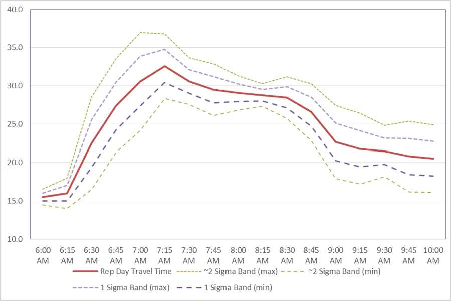

Table 11. Travel Time Variation Envelope Band Calculation, Alligator City

Time of Trip Start	Rep Day Travel Time	Standard Deviation (Sigma)	~2 Sigma Band (max)	~2 Sigma Band (min)	1 Sigma Band (max)	1 Sigma Band (min)
6:00 AM	15.5	0.53	16.5	14.5	16.0	15.0
6:15 AM	16.0	1.02	18.0	14.0	17.0	15.0
6:30 AM	22.5	3.09	28.5	16.5	25.6	19.4
6:45 AM	27.4	3.13	33.5	21.3	30.5	24.3
7:00 AM	30.6	3.26	37.0	24.2	33.9	27.3
7:15 AM	32.6	2.16	36.8	28.4	34.8	30.4
7:30 AM	30.6	1.55	33.6	27.6	32.2	29.0
7:45 AM	29.5	1.71	32.9	26.1	31.2	27.8
8:00 AM	29.1	1.14	31.3	26.9	30.2	28.0
8:15 AM	28.8	0.76	30.3	27.3	29.6	28.0
8:30 AM	28.5	1.39	31.2	25.8	29.9	27.1
8:45 AM	26.6	1.89	30.3	22.9	28.5	24.7
9:00 AM	22.7	2.44	27.5	17.9	25.1	20.3
9:15 AM	21.8	2.36	26.4	17.2	24.2	19.4
9:30 AM	21.5	1.71	24.9	18.1	23.2	19.8
9:45 AM	20.8	2.36	25.4	16.2	23.2	18.4
10:00 AM	20.5	2.25	24.9	16.1	22.8	18.2

Calibrate Model Variants within Acceptability Criteria

In the Alligator City example, consider the situation where an analyst is in the midst of calibrating the eastbound travel times from West Hills to Alligator City via the Komodo Tunnel. After a series of adjustments to the input parameters, the analyst calculates the simulated travel times for each of the 17 time intervals in the AM peak.

First, the analyst considers Criterion I to control for outliers (Figure 11). All of the points fall within the ~2 Sigma Band except for one point (8 AM). Given that there are 17 time intervals, at most one-time period can be outside the band. The model variant passes Criterion I.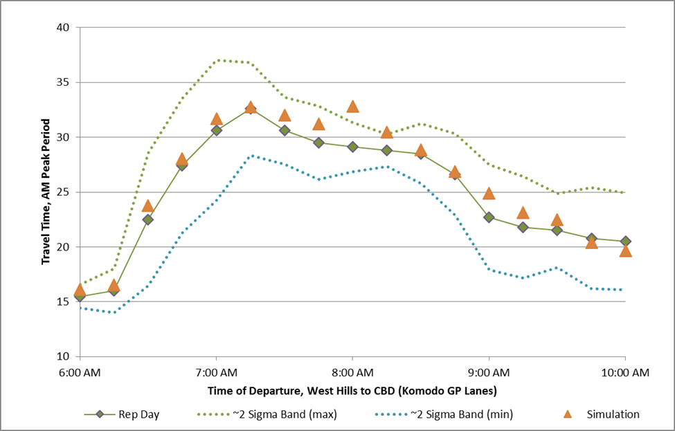

Second, the analyst considers Criterion II to control for inliers (Figure 12). All of the points fall within the 1 Sigma Band except for three points (6:00 AM, 8:00 AM, 8:15 AM). The percentage of time periods within the 1 Sigma Band is 82% (14 of 17), higher than the 66.7% requirement. Critical time periods should also be considered. For this particular measure and representative day, the peak travel time occurs at 7:15 AM. The second highest non-adjacent travel time occurs at 7:45 AM. Both the 7:15 AM and 7:45 AM simulated travel times fall within the 1 Sigma Band. Therefore, the model variant passes Criterion II.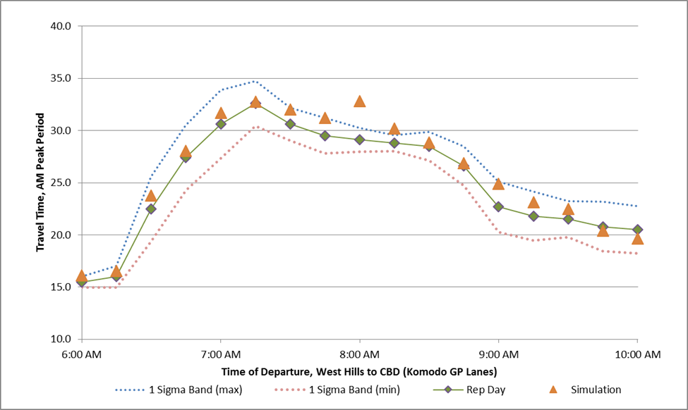

Third, the analyst computes Bounded Dynamic Absolute Error threshold for this data set using the observed travel time data from each of the other days in the cluster and the representative day. These travel times were shown previously in Figure 11, above. The BDAE threshold for these data is 1.84 minutes. Differences between the simulated travel time and observed travel time are shown in Table 12. The average absolute difference between the simulated travel times and the representative day is 1.1 minutes, less than the BDAE Threshold of 1.84. Criterion III is met.

Fourth, the analyst considers the final criteria to determine if the simulation is an unacceptably large over or under estimator of the representative day. In this case, the threshold is set to one-third of the BDAE or 0.61 minutes. If the simulation does not, on average, overestimate travel times in excess of this threshold then the criterion is met. However, the simulation does indeed provide travel times that are on average 1.0 minutes longer than the representative day. Criterion IV is not met, because the current model is an unacceptably large over-estimator of travel time. The analyst will have to continue to alter model variant parameters to meet this criterion. For some simulation models, this may mean considering a slight reduction in target vehicle speeds, either globally or along the links of this specific route. This may influence other measures and locations, however. Note that the calibration criteria are only met when a single run meets all the calibration criteria for all measures and locations. Thus, the analyst should re-examine each criterion (I, II, and III) after making an adjustment to satisfy Criterion IV.

Table 12. Assessing Criteria III and IV, Alligator City

Time of Trip Start	Simulation	Rep. Day	Absolute Diff.	Diff.
6:00 AM	16.1	15.5	0.6	-0.6
6:15 AM	16.6	16.0	0.55	-0.5
6:30 AM	23.8	22.5	1.27	-1.3
6:45 AM	28.0	27.4	0.63	-0.6
7:00 AM	31.7	30.6	1.12	-1.1
7:15 AM	32.7	32.6	0.14	-0.1
7:30 AM	32.0	30.6	1.4	-1.4
7:45 AM	31.2	29.5	1.7	-1.7
8:00 AM	32.8	29.1	3.7	-3.7
8:15 AM	30.2	28.8	1.4	-1.4
8:30 AM	28.9	28.5	0.37	-0.4
8:45 AM	26.9	26.6	0.27	-0.3
9:00 AM	24.9	22.7	2.21	-2.2
9:15 AM	23.1	21.8	1.31	-1.3
9:30 AM	22.5	21.5	0.96	-1.0
9:45 AM	20.4	20.8	0.42	0.4
10:00 AM	19.7	20.5	0.84	0.8
		AVERAGE	1.1	-1.0

Key Points

In summary, when calibrating a microsimulation study:

• Calibrate selectively, only for key performance measures.
• Performance measures for calibration should have good observed data.
• Calibrate a model variant for each travel condition.
• Use a representative day approach for calibration rather than a synthetic day combining multiple days.
• Calibration should be focused on bottleneck dynamics as well as time-variant performance measures.