Traffic Analysis Toolbox Volume III: Guidelines for Applying Traffic Microsimulation Modeling Software 2019 Update to the 2004 Version

Chapter 2. Data Collection and Analysis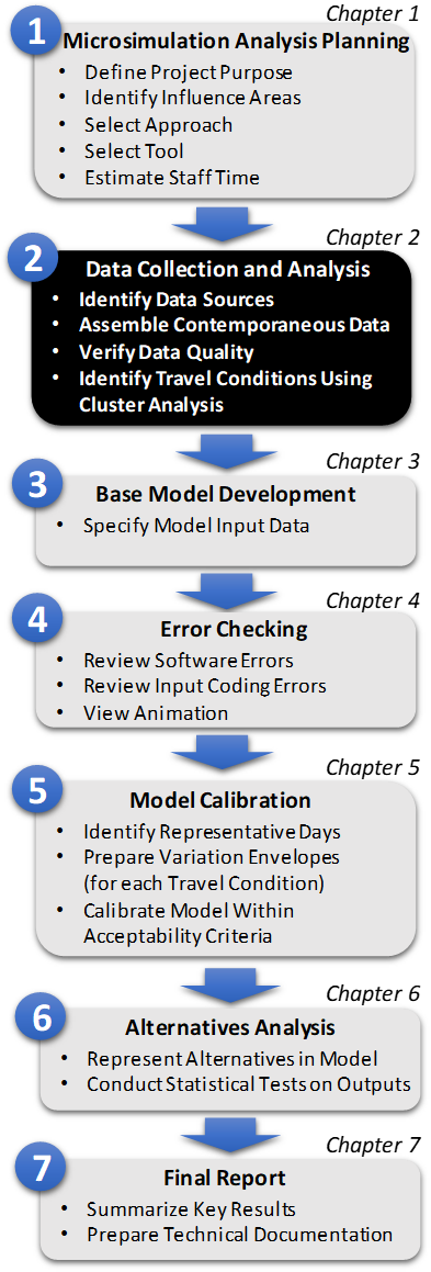

This chapter provides guidance on the identification, collection, and preparation of the data needed to develop a microsimulation model for a specific project analysis. This is Step 2 in the Microsimulation Analytical Process (Figure 4).

There are agency-specific techniques and guidance documents that focus on data collection, which should be used to support project-specific needs. These sources should be consulted regarding appropriate data collection methods. A selection of general guides on the collection of traffic data includes:

• Introduction to Traffic Engineering: A Manual for Data Collection and Analysis, T.R. Currin, Brooks/Cole, 2001, 140 pp., ISBN No. 0-534378-67-6.
• Manual of Transportation Engineering Studies, H. Douglas Robertson, Joseph E. Hummer, and Donna C. Nelson, Institute of Transportation Engineers, Washington, DC, 1994, ISBN No. 0-13-097569-9.
• Highway Capacity Manual 2010, TRB, 2010, ISBN No. 978-0-309-16077-3.
• Traffic Analysis Toolbox Volume VI - Definition, Interpretation, And Calculation of Measures of Effectiveness, R. Dowling, FHWA Report # FHWA-HOP-08-054, January 2007.
• Traffic Monitoring Guide, FHWA Report # FHWA-PL-13-015, September 2013.

Data collection can be one of the most costly components of an analytical study. It is thus essential to identify the key data that are needed for the study and budget resources accordingly. If there is limited funding, resources need to be spent judiciously so that sufficient, quality data are available for conducting a study that will inform decision makers of the potential implications of their transportation investments.

The following are the basic tenets of data collection and management for an effective analytical study using a microsimulation model:

• Use data that are measurable in the field.
• Quality and quantity of data influences analysis.
• Required analytical accuracy drives quantity collected.
• Use data that are relatively recent.
• Use data that are time variant.
• Use contemporaneous data.

An analytical study can represent the impacts of the decisionmaking process only if the model used for the study is calibrated to accurately replicate field conditions. This is feasible if data that are observable in the field are used for building and calibrating the model. Secondly, the type of analysis being conducted is dependent on the quantity and quality of data available. If the amount of available data does not adequately support the project objectives and scope identified in Task 1, then the project team should return to Task 1 and redefine the objectives and scope so that they will be sufficiently supported by the available data. The required accuracy should drive the quantity collected. Chapter 5 will discuss the approach for determining the amount of data required for a desired level of accuracy. Finally, the quality of the analysis and the resulting decisions will depend on the data that were used. Data that are relatively recent, capture the temporal variations in demand, and are concurrent should be used for a microsimulation analysis.

Until recently, due to insufficient data, analysts used a single, average day created from disparate sources and from data collected on different days. Outlier days that included incidents, weather and unusually high or low travel demand were removed from the analysis.

When making transportation investment decisions it is important to look at the cost-effectiveness of alternatives. If only a single "normal" day is used to compare the alternatives, as has been the norm for analytical studies, the effectiveness of each alternative will not be fully captured as driver behaviors vary significantly from normal to non-normal days. This makes it necessary to look at the causes and the size of the problem being addressed. For example, how many days in a year experience severe congestion? What proportion of the extreme delays can be attributed to inclement weather, such as snowstorms? What proportion of the extreme delays was caused by multi-vehicle crashes? Modeling all days, however, is not a practical approach. It is infeasible, cost-prohibitive, and unnecessary.

This version of the toolbox provides guidance on overcoming this limitation by including even the "outlier" days by assigning days into groups that experience similar travel conditions and modeling a representative day from each cluster, making it feasible cost-wise. Travel conditions are defined as a combination of operational conditions and resulting system performance. Operational conditions are identified by a combination of demand levels and patterns (e.g., low, medium or high demand), weather (e.g., clear, rain, snow, ice, fog, poor visibility), incident (e.g., no impact, medium impact, high impact), and other planned disruptions (e.g., work zones, special events) that impact system performance (e.g., travel times, bottleneck throughput).

To make wise, cost-effective investment decisions it is beneficial to identify and categorize days by travel conditions to better understand the sources of variability in the system and identify conditions when one alternative outperforms another or under what conditions an alternative is most effective. For example, to articulate the value of adaptive traffic signal control, it is critical to examine under what conditions the strategy will be most effective, and under what conditions it will not yield significant benefits. However, distinguishing between good and bad performance in a transportation system that is confounded by noise from factors such as adverse weather, incidents, etc., is challenging. Comparison of the average performance over all days in the baseline or the pre-implementation period with that in the post-implementation period will not reveal the true impacts (whether positive or negative). For example, an increase in corridor delays during the post-implementation period might be attributed to poor performance of the adaptive traffic signal control strategy. However, this might have been caused by some confounding factor, such as a series of severe weather events during the post-implementation period. Had the performance on days with severe weather events been compared, the strategy may have proved to be beneficial. Comparing the effectiveness of alternatives on similar travel conditions will help minimize the effect of confounding factors that may affect benefits analyses.

If the analyst doesn't have data for multiple days in a year that represent the possible travel conditions that a traveler may experience, then the analyst is advised to either collect data for additional days or in the event of constrained resources or schedule, explore alternative solutions to microsimulation. In recent studies, analysts have identified travel conditions by categorizing (or binning) days into pre-determined groups based on demand, and key sources of congestion for the study area being modeled. Such approaches do not accurately represent system outcomes (e.g., travel times, travel speeds, bottleneck throughput). For example, a traveler's experience on two days with identical demand and severity of incidents might not be similar if the locations of the incidents are not similar or if the number of incidents is not identical.

This chapter provides an alternate approach that makes use of cluster analysis to assign days into groups, where each group characterizes a specific travel condition. Cluster analysis helps to partition data into groups or clusters to minimize the variance within each cluster (so that days within each cluster are similar) and maximize the variance between clusters (so that days in different clusters are dissimilar). The groups are not pre-selected; instead clustering discovers natural groups that exist in the data. It should be noted that clustering does not yield a right answer. In fact, outcomes may or may not be deterministic depending on the clustering technique. Outcome of clustering is highly dependent on the pre-processing of data, selection of attributes, clustering technique, initial solution, and stopping criterion for identifying the final number of clusters.

The key steps for data collection for an analytical study include:

• Identify Data Sources.
• Assemble Contemporaneous Data.
• Verify Data Quality.
• Identify Travel Conditions Using Cluster Analysis.

Identify Data Sources

The sections below discuss the three categories of data required by an analytical study and the corresponding sources:

• Data for base model development.
• Data for determining travel conditions.
• Data for calibration.

Data for Base Model Development

The precise input data required by a microsimulation model will vary by software and the specific modeling application as defined by the study objectives and scope. Most microsimulation analytical studies will require the following types of input data:

• Road geometry (lengths, lanes, curvature).
• Traffic controls (signal timing, signs).
• Demand (entry volumes, turning volumes, O-D table).

In addition to the above basic input data, microsimulation models also require data on vehicle and driver characteristics (vehicle length, maximum acceleration rate, driver aggressiveness, etc.). Because these data can be difficult to measure in the field, it is often supplied with the software in the form of various default values. Most microsimulation tools employ statistical distributions to represent the driver and vehicle characteristics. The statistical distributions employed to represent the variability of the driver and vehicle characteristics should be calibrated to reflect local conditions.

Each microsimulation model will also require various control parameters that specify how the model conducts the simulation. The user's guide for the specific simulation software should be consulted for a complete list of input requirements. The discussion below describes only the most basic data requirements shared by the majority of microsimulation model software.

Demand data will be discussed in the data for travel conditions section.

Geometric Data

The basic geometric data required for building a model are the number of lanes, length, and design speed. For intersections, the necessary geometric data may also include the designated turn lanes, their vehicle storage lengths, and curb turn radii. These data can usually be obtained from construction drawings, field surveys, geographic information system (GIS) files, Google Maps, or aerial photographs.

Some microsimulation modeling tools may allow (or require) the analyst to input additional geometric data, such as grade, horizontal curvature, load limits, height limits, shoulders, on street parking, pavement condition, etc.

Control Data

Control data consist of the locations of traffic control devices and signal-timing settings. These data can best be obtained from the files of the agencies operating the traffic control system or from field inspection. The analyst should obtain time-stamped signal-timings when possible. A best practice is to not just rely on the information provided by the public agency. Resources should be allocated to conduct a spot-check of the data through field inspection.

Some tools may allow the inclusion of advanced traffic control features. Some tools require the equivalent fixed-time input for traffic-actuated signals. Others can work with both fixed-time and actuated-controller settings.

Vehicle Characteristics

The vehicle characteristics typically include vehicle mix, vehicle dimensions, and vehicle performance characteristics (maximum acceleration, etc.). The software-supplied default vehicle mix, dimensions, and performance characteristics should be reviewed to ensure that they are representative of local vehicle fleet data, especially for simulation software developed outside the United States.

Vehicle Mix — The vehicle mix is defined by the analyst, often in terms of the percentage of total vehicles generated in the O-D (origin-destination) process. Typical vehicle types in the vehicle mix might be passenger cars, single-unit trucks, semi-trailer trucks, and buses.

Default percentages are usually included in most software programs; however, the vehicle mix is highly localized and national default values will rarely be valid for specific locations. For example, the percentage of trucks in the vehicle mix can vary from a low of 2 percent on urban streets during rush hour to a high of 40 percent of daily weekday traffic on an intercity interstate freeway.

It is recommended that the analyst obtain one or more vehicle classification studies for the study area for the time period being analyzed. Vehicle classification studies can often be obtained from a variety of sources, including truck weigh stations, Highway performance monitoring system (HPMS), etc.

Vehicle Dimensions and Performance - The analyst should attempt to obtain the vehicle fleet data (vehicle mix, dimensions, and performance) from the local/State DOT or air quality management agency. National data can be obtained from the Motor and Equipment Manufacturers Association (MEMA), various car manufacturers, FHWA, and the U.S. Environmental Protection Agency (EPA).

Driver Characteristics

Driver characteristics typically include driver aggressiveness, reaction time, desired speeds, and acceptable critical gaps (for lane changing, merging, crossing). In addition, some tools may also allow the analyst to specify driver cooperation, awareness, and compliance (to posted speeds limits, signs, etc.).

Driver aggressiveness characterizes how drivers respond to traffic flow conditions [4]. Driver cooperation characterizes the degree to which drivers will forgo individual advantage and modify their driving behavior to assist other drivers in the traffic stream [4]. Driver awareness characterizes how informed a driver is of the traffic conditions. What percentage of the drivers are habitual drivers or commuters versus tourists? What percentage of the drivers are aware of the traffic flow conditions (e.g., queue ahead, congestion, incidents) and feasible alternatives (e.g., route, mode) through traveler information or messages posted on VMS? Driver compliance characterizes how often a driver complies with the traffic control signs, mandatory messages posted on the VMS, etc.

As is done for vehicle characteristics inputs, the software-supplied defaults should be reviewed to ensure that they are representative of the local driving population.

Traffic Operations and Management Data

Traffic operations and management data can be categorized into driver warning data, regulatory data, information (guidance) data, and surveillance detectors. For all four categories, the analyst will need the type and location of the signs or the detectors.

For warning data, the analyst will need information on the type and location of warning signs. For example, are there signs for lane drops or exits? Where are they located? For regulatory data, the analyst will need the type and location of the signs, and the information posted (e.g., regulatory speed limit in a work zone). If there are HOV lanes, the analyst will need information on the High Occupancy Vehicle (HOV) lane requirement (e.g., HOV-2 versus HOV-3), the hours, the location of signs, and information on driver compliance. If there are High Occupancy Toll (HOT) lanes, the analyst will need information on the pricing strategy and HOT management procedures. For example, the analyst may need information on how the HOT lanes are managed in the event of an incident, when and how the HOT lane requirements are modified, what the criteria are for lifting the restrictions, etc. Information or guidance data include information posted on VMS. The analyst will need the type of information that is displayed, the location, and if possible, the actual messages that were displayed. This can be obtained from the local or State DOT. The analyst will also need information on the locations of surveillance detectors.

Most of the information, including messages posted on the VMS, can be obtained from the public agency responsible for the study area. Type of signs and locations can be obtained from GIS files, aerial photographs, and construction drawings.

Data for Determining Travel Conditions

This is the second category of data that should be collected and examined when conducting an analytical study. The Verify Data Quality Section will lay out the process for identifying travel conditions through cluster analysis.

Demand Data

Travel demand data is required for both base model development as well as for identifying travel conditions.

The basic travel demand data required for most models consist of entry volumes (traffic entering the study area) and turning movements at intersections within the study area. Some models require one or more vehicular O-D tables, which enable the modeling of route diversions. An O-D table includes the number of travelers moving between different zones of a region in a defined period of time. Procedures exist in many demand modeling software and some microsimulation software for estimating O-D tables from traffic counts.

Count Locations and Duration: Traffic counts should be conducted at key locations within the microsimulation model study area for the duration of the proposed simulation analytical period. The counts should ideally be aggregated to no longer than 15-minute time periods.

If congestion is present at or upstream of a count location, care should be taken to ensure that the count measures demand and not capacity. The count period should ideally start before the onset of congestion and end after the dissipation of all congestion to ensure that all queued demand is eventually included in the count.

The counts should be conducted simultaneously if resources permit so that all count information is consistent with a single simulation period. Often, resources do not permit this for the larger simulation areas, so the analyst should establish one or more control stations where a continuous count is maintained over the length of the data collection period. The analyst then uses the control station counts to adjust the counts collected over several days, preferably for a year, into a consistent set of counts.

Estimating O-D Trip Tables: For some simulation software, the counts should be converted into an estimate of existing O-D trip patterns. Other software programs can work with either turning-movement counts or an O-D table. An O-D table is required if it is desirable to model route choice shifts within the microsimulation model.

Local metropolitan planning organization (MPO) travel demand models can provide O-D data; however, these data sets are generally limited to the nearest decennial census year and the zone system is usually too macroscopic for microsimulation. The analyst should usually estimate the existing O-D table from the MPO O-D data in combination with other data sources, such as traffic counts. This process will require consideration of O-D pattern changes by time of day, especially for simulations that cover an extended period of time throughout the day. It might be necessary to generate separate O-D tables for trucks, especially if there is significant percentage of trucks in the study area. There are many references in the literature on the estimation of O-D volumes from traffic counts [5]. Most travel demand software and some microsimulation software have O-D estimation modules available.

There are more accurate methods for measuring O-D data, including use of license plate matching survey, wireless communication data (e.g., cellular phone positioning data, data from GPS (global positioning system) enabled vehicles), etc. In the license plate matching method, the analyst establishes checkpoints within and on the periphery of the study area. License plate numbers of all vehicles passing by each checkpoint are noted either manually by the analyst or video surveillance. A matching program is then used to determine how many vehicles traveled between each pair of checkpoints. However, license plate matching surveys can be quite expensive.

In wireless communication-based methods, locations of cell phones can be derived directly from the GPS position if the phone is GPS-enabled or by tracking when a signal is received at a base station (signal tower). The locations of the cellular probes are matched to determine trip origins and destinations. To estimate the O-D matrix for a wider region, the probability of cell-phone ownership is applied. Cellular phone data can also help infer trip purpose (shopping, school, work, etc.) and mode (e.g., a slow-moving trajectory may be classified as a pedestrian).

If the study area has transit, High Occupancy Vehicles (HOV), and trucks in the vehicle mix, or if there is significant interaction with bicycles and pedestrians, the analyst will need the corresponding demand data. Even if only the peak periods are being examined, demand data should be collected before the onset of congestion and should continue until after the congestion is dissipated. To capture the temporal variations in demand it is best not to aggregate demand data to longer than 15 minutes.

For identifying travel conditions, average link flows should be calculated at two screen lines that bisect the study area. Average flows should be computed across all links that cross the screen lines. At a minimum, the average flows should be computed for the principal corridor(s) that is being modeled. Averages should be calculated for each day at 15-minute intervals; these may be averages for the entire day or just the peak periods, depending on the goals of the analysis.

Forecasting future travel demand is a challenging and difficult problem and is outside of the scope of the guidelines. Extensive literature already exists to conduct travel demand forecasts (For example, the National Cooperative Highway Research Program (NCHRP) Report 765). Analysts should bring relevant forecasting into play when conducting operations analysis for the distant future. However, given the high level of uncertainty in future demand forecasts, it may behoove the analyst to conduct sensitivity analyses around the critical uncertainties.

Weather Data

If the study area modeled experiences inclement weather, then weather data, including precipitation, rain, wind speed, snow, visibility, etc., may be obtained from the National Weather Service (NWS) [6].

Average or maximum (worst case) precipitation levels, wind speeds, and visibility should be calculated for the entire study area as a whole for each day. These may be hourly averages, average for the entire day or just the peak periods, or the maximum for the entire day or just the peak periods, depending on the goals of the analysis. For a location that experiences inclement weather frequently or for an analysis that is specifically examining impacts of weather-related strategies, the analyst should use no greater than hourly averages, and if weather data are available more frequently at intervals that match the reporting intervals for demand (e.g., 15-minute intervals), then those data should be used. But for a location that has few such occurrences, a single average, maximum or minimum for the day or the peak period may suffice depending on the needs of the analysis.

Incident Data

Incident reports should be available for the study area from the site or location's State or local department of transportation. Incidents may be classified in the incident databases by day, location, time (notification, arrival, and clearance), type (e.g., debris, non-injury collision, injury collision, disabled, police activity), impacted lanes (e.g., single lane, multiple Lanes, shoulder, HOV, total closure), and time to system recovery from incident (if available).

Incident reports should be collected for each day; these may be for the entire day or just the peak periods, depending on the goals of the analysis.

Transit Data

If the analysis includes an assessment of transit-related strategies, then average transit ridership data should be calculated for each day for bus routes traversing the study area. These may be for the entire day or just the peak periods.

Freight Data

If the analysis includes an assessment of freight strategies, then average dray orders data should be obtained for each day for principal freight routes traversing the study area. These may be for the entire day or just the peak periods.

Bottleneck Throughput

Bottlenecks are defined as an area of diminished capacity that causes congestion. Bottlenecks can be the result of physical or operational characteristics, both of which can be latent when demand is low [7]. Active bottlenecks can be further classified as either moving or stationary. An interchange or an intersection can be classified as a stationary bottleneck, while a slow-moving truck can be classified as a moving bottleneck.

At least one stationary bottleneck should be identified for the study area. Bottleneck throughput (observed counts) should be measured either immediately upstream (within 0.5 miles and prior to any major intersection or interchange) or downstream of the bottleneck. Near downstream locations are preferred, prior to the next major intersection or interchange.

Maximum bottleneck throughputs should be calculated for each day at 15-minute (or more frequent) intervals. These may be maximum throughputs for the entire day or just the peak periods, depending on the goals of the analysis.

Travel Time

Numerous methods exist in literature for estimating travel times and these may be referred for a more in-depth treatment of travel time estimation [8, 9, 10]. Highlighted here are some excerpts from the literature [8]. There are two main categories of methods for estimating travel times - those that make use of spot measurements through use of detectors and video surveillance and those that make use of probe technology.

Spot measure data collection systems directly collect speeds from vehicles passing the device. Travel times are estimated by knowing the location of the devices and the distance to the next device.

Probe vehicle techniques involve direct measurement of travel time (along a route or point-to-point) using data from a portion of the vehicle stream. In license-plate, toll tags, and Bluetooth-based methods, vehicle identification data and time stamps of vehicles passing a roadside reader device are collected and checked against the last reader passed to determine the travel time between reader locations. In wireless communication-based methods, vehicles are tracked either through cell phone triangulation using cell towers or through GPS location tracking technology.

Travel times should be measured for each day for paths that traverse the study area and intersect at least one bottleneck location. Observed data should be available for these measures at 15-minute (or more frequent) intervals. More than one path may be required to capture the system dynamic. For example, for corridor analyses, the mainline and one alternative path are required. An interchange analysis may require only one path.

Data for Calibration

Additional data may be needed for calibrating the model. Calibration is the process of systematically adjusting model parameters so that the model emulates observed traffic conditions at the study area. To determine if the model represents the observed traffic conditions, the analyst will need to identify key calibration performance measures and the data needed for estimating these performance measures. The analyst should choose at least two key measures for an effective calibration.

Calibration performance measures fall into two broad categories: 1. Localized (i.e., segment-level or intersection-level) performance, 2. System (i.e., route-level, corridor level, or system-level) performance.

At a minimum, the analyst should calibrate to at least one localized performance measure and one system performance measure. The localized measure should capture bottleneck dynamics. Examples of such measures include, bottleneck throughput or duration, density, queuing. For system performance measure, the analyst may select travel time or speed profiles along one or more key routes on the roadway network. The analyst may also choose to calibrate to additional performance measures depending on the objective of the study and the need to differentiate between the alternatives being examined in the study. For example, for designing or evaluating a traffic signal system, queue lengths, intersection delays, and turning percentages may be selected as additional calibration performance measures.

Assemble Contemporaneous Data

For each category of data identified in the previous section, contemporaneous data should be collected for the entire study period (preferably a year). For example, if demand data are collected for year 2014, control data, incident and weather data should also be collected for year 2014. If all the data are not collected over the same time frame, there may be problems resolving data inconsistencies or in calibrating the model. For example, estimating freeway travel times during the AM peak, and demand and incident information during the PM peak will make calibration challenging.

Verify Data Quality

Several methods for error checking have been cited in the literature and these should be consulted by the analyst [7, 11]. Resources should be allocated for the analyst to verify the data through field inspection and surveys. This section identifies some key data quality checks the analyst may perform:

Some examples of localized calibration performance measures are: bottleneck throughput, bottleneck duration, extent of queues at bottleneck, segment-level speed profiles, number of stops, intersection delays, turning percentages, etc.

Examples of system calibration performance measures are: travel times travel time index, planning index, travel time variance, network or route specific delays, etc.

There is comprehensive treatment of measurement of speeds, stops, queues, delays, density, travel time variance, etc., using field data in the literature [9] and hence will not be discussed in this section.

If using an existing model that was calibrated several years ago, the analyst will have to re-calibrate the model. In that case, the analyst will need to collect data not only for estimating calibration performance measures but also demand data. The analyst will need to further verify if geometric data, traffic control data and traffic operations and management data are still accurate and valid.

• Spot-check of geometric, control and traffic operations and management data should be done through field inspections to confirm if the files obtained match what is in the ground.
• Geometric and control data should be reviewed for apparent violations of design standards and/or traffic engineering practices. Sudden breaks in geometric continuity (such as a short block of a two-lane street sandwiched in between long stretches of a four-lane street) may also be worth checking with people who are knowledgeable about local conditions. Breaks in continuity and violations of design standards may be indicative of data collection errors.
• Internal consistency of counts should be reviewed. Upstream counts should be compared to downstream counts. Unexplained large jumps or drops in the counts should be reconciled. There is no guidance on precisely what constitutes a "large" difference in counts. The analyst might consider investigating any differences of greater than 10 percent between upstream and downstream counts for locations where no known traffic sources or sinks (such as driveways) exist between the count locations. Larger differences are acceptable where driveways and parking lots could potentially explain the count differences.
• Travel time and speed data obtained from probe vehicle techniques should be reviewed for realistic segment travel times and speeds.
• Discrepancies in counts resulting from counting errors or counts made on different days should be reconciled before proceeding to the model development task. Inconsistent counts make error checking and model calibration much more difficult. That is why it is critical to obtain concurrent or contemporaneous data.

Identify Travel Conditions Using Cluster Analysis

This section describes the steps for conducting an effective cluster analysis to identify travel conditions that are revealed by the data.

Step 1: Identify Attributes

The goal of this step is to identify key attributes for defining the travel conditions experienced at the site. Travel conditions should be represented by demand, sources of congestion for the site, and key system outcomes or performance (e.g., bottleneck throughput, travel times). Later on, in Chapter 5, this characterization of system performance will be critical in assessing whether the simulation tool is calibrated enough to well represent the portfolio of travel conditions. Example attributes are listed below:

• Demand.
• Weather.
• Incident.
• Transit.
• Freight.
• Bottleneck Throughput.
• Travel Time.

Sources of data required for each attribute are discussed in the Data for Determining Travel Conditions Section. After collecting concurrent data and verifying the data quality, proceed to Step 2.

Step 2: Process Data

All qualitative data should be transformed into quantitative or numeric data. However, it is crucial to not over process the qualitative data so that there are only a couple of indices that fail to capture the relationship between the attribute and the key measure of interest. For example, incidents should not be reduced to just three levels, representing a no-incident situation, low severity incident, and high severity incident based on closure time and number of impacted lanes. Two days might be assigned a low severity index if the two days had an incident on one lane for less than 30 minutes. What if one of the days had multiple small incidents that together amounted to a closure of 30 minutes within the peak period, while the other had a single incident that lasted the entire 30 minutes? Alternately, what if the type of incident on one day is a fatality while on the other day is a non-injury multi-vehicle collision? Will the rubbernecking experienced on adjacent lanes be the same? That is why it is not recommended to do categorization up front without assessing the impact of these incidents - i.e., without including travel times and/or bottleneck throughput in the clustering. It is best to just transform the data onto a numeric scale and let the cluster analysis decide which cluster/group the day fits into. One approach for transforming qualitative data is by defining a numeric scale that is exhaustive (i.e., considers all combinations observed in the data). For example, the analyst may want to define a numeric scale that looks at all combinations of the following incident-related attributes:

• Type of incident.
• Number of impacted lanes.
• Location of incident: This can be done by specifying if the incident occurs upstream of the natural bottleneck, downstream of the bottleneck, or at the bottleneck. Alternately, the location can be specified as the distance from the natural bottleneck.
• Time of occurrence: Here the analyst can specify if the incident occurs prior to the peak period, during the peak period, or after the peak period. Alternately, the analyst can specify the time of occurrence as the difference in time expressed in hours (rounded up) from the start of the simulation period. For example, if the peak period is from 6 to 9 AM, the analyst might choose a simulation period of 5 to 10 AM. If an incident occurs at 8:30 AM, the time of occurrence can be expressed as 4, as the incident occurs in the 4th hour after the start of the simulation period.
• Clearance or closure time: This should be a factor of what is observed in the data. This may be expressed in increments of 5, 10, or 15 minutes. But if it typically takes 15 minutes or more for clearance, there is no need to define in increments of 5 or 10 minutes.

Numeric data should not be further reduced into bins or categories. So, if weather data includes precipitation, the analyst should use the precipitation levels without further reducing them into two levels to represent no rain (0 mm) and rain (> 0mm). If only qualitative information is available (e.g., snow, blowing snow, sleet, etc.), then the analyst should define a numeric scale that includes all observed data for that category. An alternate approach is to transform categorical data to a binary scale.

Note that some clustering tools have built-in solutions to deal with categorical variables.

Step 3: Normalize Data

Once qualitative data are transformed onto a numeric scale, all data (numeric as well as qualitative data that have been transformed) should be normalized. Data that are measured on different numeric scales are normalized or converted to a common scale so that no single attribute dominates the others. Normalization is done using the following equation:

\(x^{'} = a + \frac{\left( x - x_{\min} \right)\left( b - a \right)}{x_{\max} - \ x_{\min}}\)(1)

where:

x': normalized value of data x

x_min: minimum value for the attribute (min over all x)

x_max: maximum value for the attribute (max over all x)

a: minimum value of common scale (e.g., 0 if normalizing to scale of 0 to 1)

b: maximum value of common scale (e.g., 1 if normalizing to scale of 0 to 1)

It should be noted that some of the tools will do this for you.

Step 4: Down select Attributes

After data have been normalized, the analyst should filter out those attributes that are either redundant or have no impact on the key measure of interest (e.g., travel time, bottleneck throughput). It is best to use attributes that are highly correlated with the key measure of interest but have low correlation with each other. Highly correlated attributes effectively represent the same phenomenon. Hence, if highly correlated attributes are included, then that phenomenon will dominate the other attributes thereby skewing the cluster analysis. So, for example, if the incident attributes are highly correlated with each other, select the attribute from the set of correlated incident attributes, which has the most impact on travel times. Most clustering tools have a built-in capability or algorithm to filter out redundant attributes or reduce the dimensionality (i.e., if there are too many attributes). One commonly used algorithm for dimensionality reduction is Principal Component Analysis (PCA), which converts a set of possibly correlated observations into a set of linearly uncorrelated variables called principal components.

Step 5: Perform Clustering

There are several clustering techniques and heuristics for discrete and continuous data. Examples of statistical and data mining tools that offer clustering capability are the commercial tools such as, MATLAB [12], IBM SPSS [13], and SAS [14], or the open source software such as, WEKA [15] (Waikato Environment for Knowledge Analysis), GNU Octave [16], R [17], Apache Spark MLlib [18], H2O [19], and TensorFlow [20].

Examples of commonly used clustering techniques are K-means, hierarchical clustering, and expectation maximization. These have been well-documented in the literature and are not discussed here.

Step 6: Identify Stopping Criterion

Data mining tools have inbuilt stopping criterion. Some tools use cross-validation to determine the optimal cluster size. The analyst can also select one of the several heuristics from the literature for determining when to stop the clustering. Given below is one such simple heuristic for determining the stopping criterion.

1. Set the maximum cluster size as \(2 \times \sqrt{n/2}\) where n is the number of days.
2. Set k= 3 (initial cluster size).
3. Perform clustering using k clusters.
4. Calculate either of the following functions for the key measure of interest (e.g., travel times, bottleneck throughput).

   Option 1:

   Within Cluster Variance \(/\) Between Cluster Variance(2)

   Option 2:

   Coefficient of Variation Normalized over all clusters × # of Clusters Normalized between 3 and \(2 \times \sqrt{n/2}\)(3)

5. Repeat steps 3 and 4 by systematically incrementing k by 1 until the maximum cluster size is reached.
6. Select the optimal cluster size as the size of the cluster that minimizes the function in step 4.

This process can be extended to include a weighted combination of key measures of interest and locations.

Example Problem: Data Collection and Analysis

This section walks through the data collection and analysis process for the Alligator City example problem discussed in Chapter 1. The analyst should identify, collect, and clean the data for the Alligator City network for the AM peak.

Identify Data Sources

The AM peak period is designated to be from 6 to 9 AM. Data are collected from 5 to 10 AM to allow for congestion to build up and dissipate. Data are available from 10 detector stations and a cell-phone tracking study. Data have been archived for the past 1 year.

Geometric Data: GIS files, Google Maps, construction drawings, and field inspections are used to obtain the lengths and the number of lanes for each section of the Alligator City network, including the Marine Causeway, Victory Island Bridge, Komodo Tunnel, Riverside Parkway, and the Alligator City CBD (Central Business District). Turn lanes and pocket lengths are determined for each intersection in the CBD.

Transition lengths for lane drops and additions are determined. Lane widths are measured if they are not standard widths. Horizontal curvature and curb return radii are determined if the selected software tool is sensitive to these features of the road and freeway design. Free-flow speeds are estimated based on the posted speed limits for the freeway and the surface streets.

Control Data: Signal settings are obtained from Alligator City's records for an entire year, and verified in the field. The signals in Alligator City are fixed-time, having a cycle length of 90 s.

Vehicle Characteristics Data: As truck traffic is heavy, truck percentages are obtained from the Alligator City DOT. Truck performance and classifications are obtained from the Intermodal facility. For the rest of the vehicle characteristics defaults provided with the microsimulation software are used in this analysis.

Driver Characteristics Data: The default driver characteristics provided with the microsimulation software are used in this analysis.

Traffic Operations and Management Data: As there are HOV and HOT lanes, the lane requirement, hours when active, pricing strategy, and location of signs are obtained. As trucks are restricted on the ramp from Victory Island Bridge to the Riverside Parkway, truck restriction information including, location of signs, and hours when active are obtained. The location and content of the VMS posted on the Marine Causeway are obtained. All data are obtained from the Alligator City agency records.

Demand Data: Data from a cell-phone tracking study are available for the Alligator City Metropolitan area. The cell-phone location data are used to estimate 15-minute interval O-D trip tables for the region.

In addition, for identifying travel conditions a screen line is drawn across the Marine Causeway at detection station 2, which is located at the entrance of the Eastbound Marine Causeway. Average flows are calculated at 15-minute intervals for the AM peak period at detector station 2.

Weather Data: Precipitation levels and wind speeds are obtained from the NWS website for Alligator City. Visibility data was not available for the entire time period.

Incident Data: Incident type and the lanes blocked are available and these are collected for the entire year.

Bottleneck Throughput: Three bottlenecks are identified for the Alligator City network:

• Marine Causeway to Victory Island Bridge.
• Victory Island Bridge Exit at Moseley Street to the Alligator City CBD.
• Komodo Tunnel Exit at Osceola Avenue to the Alligator City CBD.

Counts are measured approximately 0.5 miles upstream of the bottlenecks at detector stations 7, 8, 9 and 10 at 15-minute intervals.

Travel Time: Travel times are estimated using the cell-phone tracking study data at 15-minute intervals for the following three paths:

• West Hills to the CBD via the Victory Island Bridge.
• West Hills to the CBD via the Tunnel using General Purpose Lanes.
• West Hills to the CBD via the Tunnel using HOV Lanes.

Calibration Data: The model will be calibrated against estimates of bottleneck throughput and travel times.

Assemble Contemporaneous Data and Verify Data Quality

The input data are reviewed by the analyst for consistency and accuracy prior to data entry. The turning, ramp, and freeway mainline counts are reconciled by the analyst to produce a set of consistent counts for the entire study area. After completion of the reconciliation, all volumes discharged from upstream locations are equal to the volumes arriving at the downstream location.

Example Cluster Analysis Using the K-Means Algorithm

Given below are the steps for conducting cluster analysis using the k-means clustering algorithm. The k-means algorithm is a widely used cluster analysis algorithm, which aims to partition n observations into k clusters such that each observation belongs to the cluster with the closest mean. The partitioning is done by minimizing the sum of squares of distances between the observations and the cluster centroids. The k-means algorithm is one of the simplest clustering algorithms, but it is computationally difficult. Several efficient heuristic algorithms that converge quickly have been developed to overcome this limitation. One of these heuristics is described below [20]. Despite being commonly used, the k-means algorithm has a few drawbacks:

• The number of clusters k is pre-defined. An inappropriate choice of k may yield poor results.
• Convergence to a local minimum may produce counterintuitive results.
• The clustering algorithm is such that all data, including outliers, are assigned to a cluster.

The k-means clustering algorithm is used here only for the purpose of introducing the cluster analysis concept. Other algorithms, such as Expectation Maximization (EM) and Hierarchical clustering, which address some of the weaknesses listed may be used in lieu of the k-means algorithm.

There are two types of hierarchical clustering algorithms — agglomerative and divisive. In agglomerative clustering, each observation starts in its own cluster and pairs of clusters that are similar are successively merged until all clusters have been merged into a single cluster. In divisive clustering, all observations start off in one cluster, and clusters are successively split until each cluster has only one observation. The advantage of the hierarchical clustering is that the number of clusters do not need to be pre-defined. The user can determine when to stop based on a pre-defined stopping criterion. The disadvantage is that it is time consuming. The EM algorithm is similar to k-means, but uses probabilities to assign data to clusters. The goal is to maximize the probability that the data falls into the clusters created. The main advantage of the EM algorithm is that it is robust to noisy data. It is able to cluster data even when incomplete. The main disadvantage is that it converges very slowly.

Each step is illustrated using the Alligator City hypothetical simulation study as an example. The guidance provided here is intended to give general advice on clustering using k-means. For simplicity, data for only a month is shown throughout the example. The tables show only a single entry for each attribute for each day. The analyst should collect data for a longer period of time, such as a year, and should include data at 15-minute or hourly intervals depending on the observed variation for that attribute. For example, if there is very little precipitation throughout the year, there is no need to include precipitation at 15-minute or hourly intervals. A single value corresponding to the maximum precipitation levels observed during the 24-hour period or the peak period may be used. But for localized and system performance measures, such as bottleneck throughput and travel times, it is essential to use time-variant measures to capture the variability in the data. Hence, for these "attributes" the analyst should use measures estimated at 15-minute (or more frequent) intervals for each day in the cluster analysis.

Step 1: Identify Attributes

Table 1 shows the data assembled for the AM Peak which extends from 6 AM to 9 AM.

Table 1. Data Assembled for Travel Conditions Identification (Step 1)

Day	Day of Week	AM Peak (6-9 AM) Demand (vph)	AM Peak (6-9 AM) Weather		AM Peak (6-9 AM) Incident		AM Peak (6-9 AM) Travel Time (min)			AM Peak (6-9 AM) Bottleneck Throughput (vph)
		Detector #2; Avg. Count (vph)	Precipitation (mm)	Wind Speed (mph)	Incident Type	Lanes Blocked	WH to CBD (VIB)	WH to CBD (Tunnel-GP)	WH to CBD (Tunnel-HOV)	Marine Causeway-V.I.Bridge Link	V. I. Bridge Exit at Moseley Street	Komodo Tunnel Exit at Osceola Ave
2-Jan-12	2	4650	0.034	4.54	Disabled	Single Lane	36	32	27	2525	1934	2042
3-Jan-12	3	4557	0.192	5.62	Non-Injury Collision	Single Lane	46	39	33	2015	1767	1652
4-Jan-12	4	4253	0.006	4.34	Debris	Multiple Lane	44	35	30	2478	1835	1760
5-Jan-12	5	5126	0.016	4.77	Non-Injury Collision	Shoulder/Median	26	24	21	2756	2105	2344
6-Jan-12	6	3529	0.04	6.18	Debris	Multiple Lane	43	36	32	2013	1843	1742
16-Jan-12	2	2875	0.07	1.55	Non-Injury Collision	HOV	49	40	36	1524	1690	1594
17-Jan-12	3	2783	0	3.08	Injury Collision	Single Lane	51	44	38	2183	1664	1418
18-Jan-12	4	3071	0.034	4.60	Disabled	Single Lane	35	32	28	1735	1956	2052
19-Jan-12	5	4348	0.298	6.13	Debris	Multiple Lane	44	36	32	1957	1820	1720
20-Jan-12	6	4119	0	3.39	Debris	Single Lane	30	27	22	2517	2084	2258
23-Jan-12	2	3799	0.37	10.23	Abandoned Vehicle	Shoulder/Median	60	53	42	2352	1550	1287
24-Jan-12	3	4872	0.076	1.70	Disabled	HOV	40	34	33	1753	1919	1943
25-Jan-12	4	3302	0	4.73	Disabled	Shoulder/Median	26	22	21	1586	2166	2431
26-Jan-12	5	3952	0	2.39	Non-Injury Collision	Single Lane	46	39	32	1957	1796	1681
27-Jan-12	6	3913	0	1.77	Abandoned Vehicle	Shoulder/Median	56	52	41	2722	1551	1272
30-Jan-12	2	4052	0.014	2.23	Debris	Multiple Lane	43	34	31	2723	1858	1795
31-Jan-12	3	4704	0	4.01	Disabled	Single Lane	35	32	28	1694	1940	2033

Step 2: Process Data

The next step is to transform qualitative attributes to a quantitative scale. In the example in Table 1, an incident is defined by type and impacted lanes. The two incident attributes are reduced to a numeric value that represents the incident severity (Table 2). Table 3 presents the data that have been transformed onto a quantitative scale. Similar such rules should be developed for transforming qualitative data into quantitative data.

Table 2. Example Transformation of Incident Qualitative Data into Numeric Data (Step 2)

Incident Type	Lanes Blocked	Severity Index
Abandoned	Shoulder/Median	1
Disabled	Shoulder/Median	2
Non-Injury Collision	Shoulder/Median	3
Debris	Single Lane	4
Debris	HOV	5
Disabled	Single Lane	6
Disabled	HOV	7
Debris	Multiple Lanes	8
Non-Injury Collision	Single Lane	9
Non-Injury Collision	HOV	10
Injury Collision	Single Lane	11
Injury Collision	HOV	12
Injury Collision	Multiple Lanes	13

Step 3: Normalize Data

Data are normalized onto a scale of 0 to 1 using equation 1. Table 4 presents the normalized data.

Step 4: Down Select Attributes

In the example, visibility data was not available for the entire period, and when available it was found to be highly correlated with the precipitation. So, visibility was eliminated from the analysis. The other attributes were not highly correlated.

Table 3. Transforming Qualitative Data onto Quantitative Scale (Step 2)

DAY	Day of Week	AM Peak (6-9 AM) Demand	AM Peak (6-9 AM) Weather		AM Peak (6-9 AM) Incident Severity	AM Peak (6-9 AM) Travel Time (min)			AM Peak (6-9 AM) Bottleneck Throughput (vph)
		Detector #2; Avg. Count (vph)	Precipitation(mm)	Wind Speed (mph)		WH to CBD (VIB)	WH to CBD (Tunnel-GP)	WH to CBD (Tunnel-HOV)	Marine Causeway-V.I.Bridge Link	V. I. Bridge Exit at Moseley Street	Komodo Tunnel Exit at Osceola Ave
2-Jan-12	2	4,650	0.034	4.54	6	36	32	27	2525	1934	2042
3-Jan-12	3	4,557	0.192	5.62	9	46	39	33	2015	1767	1652
4-Jan-12	4	4,253	0.006	4.34	8	44	35	30	2478	1835	1760
5-Jan-12	5	5,126	0.016	4.77	3	26	24	21	2756	2105	2344
6-Jan-12	6	3,529	0.04	6.18	8	43	36	32	2013	1843	1742
16-Jan-12	2	2,875	0.07	1.55	10	49	40	36	1524	1690	1594
17-Jan-12	3	3,051	0	3.08	11	51	44	38	2183	1664	1418
18-Jan-12	4	3,029	0.034	4.60	6	35	32	28	1735	1956	2052
19-Jan-12	5	4,605	0.298	6.13	8	44	36	32	1957	1820	1720
20-Jan-12	6	4,737	0	3.39	4	30	27	22	2517	2084	2258
23-Jan-12	2	3,294	0.37	10.23	13	60	53	42	2352	1550	1287
24-Jan-12	3	4,492	0.076	1.70	7	40	34	33	1753	1919	1943
25-Jan-12	4	3,618	0	4.73	2	26	22	21	1586	2166	2431
26-Jan-12	5	4,772	0	2.39	9	46	39	32	1957	1796	1681
27-Jan-12	6	2,736	0	1.77	13	56	52	41	2722	1551	1272
30-Jan-12	2	3,494	0.014	2.23	8	43	34	31	2723	1858	1795
31-Jan-12	3	4,396	0	4.01	6	35	32	28	1694	1940	2033

Table 4. Normalizing Data (Step 3)

DAY	Day of Week	AM Peak (6-9 AM) Demand	AM Peak (6-9 AM) Weather		AM Peak (6-9 AM) Normalized Incident Severity	AM Peak (6-9 AM) Normalized Travel Time			AM Peak (6-9 AM) Normalized Bottleneck Throughput
		Normalized Detector #2 Avg. Count	Normalized Precipitation	Normalized Wind Speed		WH to CBD (VIB)	WH to CBD (Tunnel-GP)	WH to CBD (Tunnel-HOV)	Marine Causeway- V.I.Bridge Link	V. I. Bridge Exit at Moseley Street	Komodo Tunnel Exit at Osceola Ave
2-Jan-12	2	0.80	0.09	0.34	0.36	0.29	0.32	0.29	0.81	0.62	0.66
3-Jan-12	3	0.76	0.52	0.47	0.64	0.59	0.55	0.57	0.40	0.35	0.33
4-Jan-12	4	0.63	0.02	0.32	0.55	0.53	0.42	0.43	0.77	0.46	0.42
5-Jan-12	5	1.00	0.04	0.37	0.09	0.00	0.06	0.00	1.00	0.90	0.92
6-Jan-12	6	0.33	0.11	0.53	0.55	0.50	0.45	0.52	0.40	0.48	0.41
16-Jan-12	2	0.06	0.19	0.00	0.73	0.68	0.58	0.71	0.00	0.23	0.28
17-Jan-12	3	0.13	0.00	0.18	0.82	0.74	0.71	0.81	0.53	0.19	0.13
18-Jan-12	4	0.12	0.09	0.35	0.36	0.26	0.32	0.33	0.17	0.66	0.67
19-Jan-12	5	0.78	0.81	0.53	0.55	0.53	0.45	0.52	0.35	0.44	0.39
20-Jan-12	6	0.84	0.00	0.21	0.18	0.12	0.16	0.05	0.81	0.87	0.85
23-Jan-12	2	0.23	1.00	1.00	1.00	1.00	1.00	1.00	0.67	0.00	0.01
24-Jan-12	3	0.73	0.21	0.02	0.45	0.41	0.39	0.57	0.19	0.60	0.58
25-Jan-12	4	0.37	0.00	0.37	0.00	0.00	0.00	0.00	0.05	1.00	1.00
26-Jan-12	5	0.85	0.00	0.10	0.64	0.59	0.55	0.52	0.35	0.40	0.35
27-Jan-12	6	0.00	0.00	0.02	1.00	0.88	0.97	0.95	0.97	0.00	0.00
30-Jan-12	2	0.32	0.04	0.08	0.55	0.50	0.39	0.48	0.97	0.50	0.45
31-Jan-12	3	0.69	0.00	0.28	0.36	0.26	0.32	0.33	0.14	0.63	0.66

Step 5: Perform Clustering

Step 5.1: Sort data by bottleneck throughput at any one critical location. In the example, the tunnel to the Osceola Ave. exit is used as the critical location. If desired, data may be sorted again over travel time for a critical trip. Sorting is done to reach convergence quickly in Step 5.6.

Step 5.2: Specify the initial number of clusters, k as 3.

Step 5.3: Divide the days systematically into k clusters with nearly equal number of days. In our example, the 17 days can be divided into three clusters, with two clusters having 6 days and one cluster having 5 days. Table 5 presents the data that have been sorted and partitioned into 3 clusters.

Step 5.4: Calculate the centroid or the mean of each cluster. Means are calculated for each attribute. In the example, we make the assumption that each attribute has the same weight. But this can be changed so that one attribute has a higher weight implying that it contributes to the grouping or clustering more than the others. Table 6 presents the centroids or means of each cluster for each attribute.

Step 5.5: Calculate the Euclidean distance of each data to the centroids of the k clusters. This is done using the following equation:

\(\text{xdis}_{y} = \sqrt{{(x_{1} - \text{ymean}_{1})}^{2} + {(x_{2} - \text{ymean}_{2})}^{2} + {(x_{3} - \text{ymean}_{3})}^{2} + \ldots}\)(4)

where:

\(\text{xdis}_{y\ }:\) distance of data x to mean of cluster y

\(x_{1\ }:\) value corresponding to attribute 1 for data x

\(\text{ymean}_{a}\)_: mean value for attribute a for cluster y

Step 5.6: Assign each day to the cluster which has the closest centroid. Table 7 shows the distances of each data to the cluster centroids and assigns them to a new cluster, which is the nearest cluster. As highlighted in Table 7, in Iteration 1, January 3^rd and 26^th were re-assigned from cluster 1 to cluster 2 and January 18^th was re-assigned from cluster 3 to cluster 2 since they were closest to the cluster 2 centroid. All other days remained in their previous clusters.

Step 5.7: If there is no change in the cluster, stop and proceed to Step 6. Otherwise, repeat steps 5.4-5.7. In the example, since there was a change, we go back to Step 5.4 and continue the process.

Step 6: Identify Stopping Criterion: In the example, we apply option 1 (see Eq. 2).

1. Set the maximum cluster size as \(2 \times \sqrt{n/2}\). In our example, we only used 17 days. So, the maximum size is 6.
2. Set k= 3 (initial cluster size).
3. Perform clustering using k clusters (which was done in Step 5).
4. The key measure of interest may be chosen as the bottleneck throughput at the Komodo tunnel to Osceola Ave exit. Calculate the function given in Eq. 2.
5. Repeat steps 6.3 and 6.4 by systematically incrementing k by 1 until the maximum cluster size (6 in the example) is reached.
6. Select the cluster size that minimizes the function calculated in step 6.5 across all cluster sizes.

Table 5. Iteration 0 - Preliminary Assignment of Data into Clusters (Step 5.3)

DAY	Day of Week	AM Peak (6-9 AM) Demand (vph)	AM Peak (6-9 AM) Weather		AM Peak (6-9 AM) Normalized Incident Severity	AM Peak (6-9 AM) Normalized Travel Time			AM Peak (6-9 AM) Normalized Bottleneck Throughput			Cluster
		Normalized Detector #2 Avg. Count	Normalized Precipitation	Normalized Wind Speed		WH to CBD (VIB)	WH to CBD (Tunnel-GP)	WH to CBD (Tunnel-HOV)	Marine Causeway-V.I.Bridge Link	V. I. Bridge Exit at Moseley Street	Komodo Tunnel Exit at Osceola Ave
27-Jan-12	6	0.00	0.00	0.02	1.00	0.88	0.97	0.95	0.97	0.00	0.00	1
23-Jan-12	2	0.23	1.00	1.00	1.00	1.00	1.00	1.00	0.67	0.00	0.01	1
17-Jan-12	3	0.13	0.00	0.18	0.82	0.74	0.71	0.81	0.53	0.19	0.13	1
16-Jan-12	2	0.06	0.19	0.00	0.73	0.68	0.58	0.71	0.00	0.23	0.28	1
3-Jan-12	3	0.76	0.52	0.47	0.64	0.59	0.55	0.57	0.40	0.35	0.33	1
26-Jan-12	5	0.85	0.00	0.10	0.64	0.59	0.55	0.52	0.35	0.40	0.35	1
19-Jan-12	5	0.78	0.81	0.53	0.55	0.53	0.45	0.52	0.35	0.44	0.39	2
6-Jan-12	6	0.33	0.11	0.53	0.55	0.50	0.45	0.52	0.40	0.48	0.41	2
4-Jan-12	4	0.63	0.02	0.32	0.55	0.53	0.42	0.43	0.77	0.46	0.42	2
30-Jan-12	2	0.32	0.04	0.08	0.55	0.50	0.39	0.48	0.97	0.50	0.45	2
24-Jan-12	3	0.73	0.21	0.02	0.45	0.41	0.39	0.57	0.19	0.60	0.58	2
31-Jan-12	3	0.69	0.00	0.28	0.36	0.26	0.32	0.33	0.14	0.63	0.66	2
2-Jan-12	2	0.80	0.09	0.34	0.36	0.29	0.32	0.29	0.81	0.62	0.66	3
18-Jan-12	4	0.12	0.09	0.35	0.36	0.26	0.32	0.33	0.17	0.66	0.67	3
20-Jan-12	6	0.84	0.00	0.21	0.18	0.12	0.16	0.05	0.81	0.87	0.85	3
5-Jan-12	5	1.00	0.04	0.37	0.09	0.00	0.06	0.00	1.00	0.90	0.92	3
25-Jan-12	4	0.37	0.00	0.37	0.00	0.00	0.00	0.00	0.05	1.00	1.00	3

Table 6. Calculating Cluster Means (Step 5.4)

Centroid	Demand	Precipitation	Wind Speed	Incident Type	Travel Time from WH to CBD (VIB)	Travel Time from WH to CBD (Tunnel-GP)	Travel Time from WH to CBD (Tunnel- HOV)	Throughput at Marine Causeway-V. I. Bridge Link	Throughput at V. I. Bridge Exit at Moseley Street	Throughput at Komodo Tunnel Exit at Osceola Ave
Cluster 1	0.34	0.28	0.29	0.80	0.75	0.73	0.76	0.49	0.19	0.18
Cluster 2	0.58	0.20	0.29	0.50	0.46	0.40	0.48	0.47	0.52	0.48
Cluster 3	0.63	0.05	0.33	0.20	0.14	0.17	0.13	0.57	0.81	0.82

Key Points

The guidance leverages use of concurrent data for supporting the analysis. In areas, where these data are not available, it is recommended that either the necessary concurrent data be collected or an alternate analytical technique in lieu of microsimulation analysis be considered. In summary, when collecting data:

• Measure flows and estimate or forecast demand.
• Temporal and geographic scope will impact estimation of demand; so broaden scope to account for onset and dissipation of congestion.
• Ensure flow conservation since it influences analysis.
• Use up-to-date GIS files, maps and drawings.
• Collect contemporaneous data.
• Errors in data will make calibration challenging; so ensure data are accurate and verify with field inspection.