Traffic Analysis Toolbox Volume III: Guidelines for Applying Traffic Microsimulation Modeling Software 2019 Update to the 2004 Version

Chapter 3. Base Model Development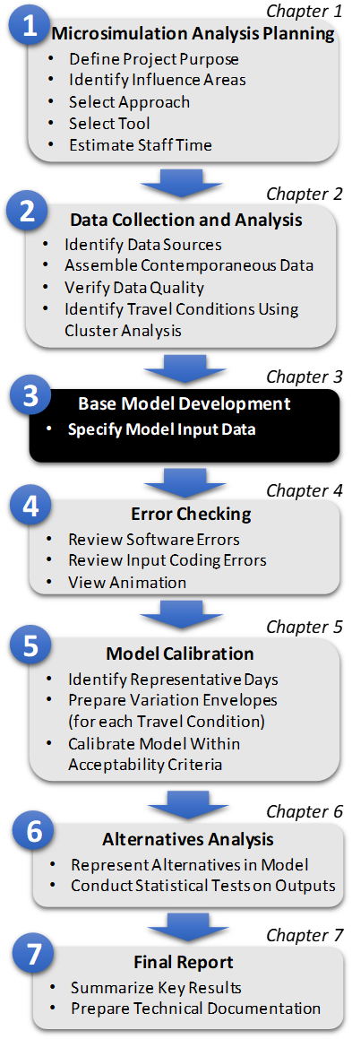

This chapter provides general guidance on the procedures for developing a microsimulation model. This is Step 3 in the Microsimulation Analytical Process (Figure 5). In this step, the analyst should develop base models for all travel conditions or clusters identified in Chapter 2. A complete operational analysis using a full year of data is a useful step to making effective investment decisions. However, when resources are constrained, it may not be cost effective to model every condition. The analyst may want to model only those travel conditions where alternatives are likely to have significant impacts. In fact, these subset of travel conditions may be further clustered to distinguish the nuances between the alternatives. For example, when assessing two weather-related alternatives, the analyst may want to further cluster the weather-related data and model only those clusters. There are many software tools for performing this task and each has its own unique method to build the model. The guidance provided here is intended to give general advice on model development; however, the analyst should consult the specific microsimulation software documentation for information on available data input tools and techniques.

Specify Model Input Data

Building a model is analogous to building a house. You begin with a blueprint and then you build each element in sequence-the foundation, the frame, the roof, the utilities and drywall, and finally the interior details. The development of a successful simulation model is similar in that you should begin with a blueprint (the link- node diagram) and then you proceed to build the model in sequence-coding links and nodes, filling in the link geometries, adding traffic control data at appropriate nodes, coding travel demand data, adding traveler behavior data, and finally selecting the model run control parameters. Any assumptions, default values or deviations from defaults values should be discussed and incorporated into the Methods and Assumptions document of the project for examination and cross-validation.

Link-Node Diagram: Model Blueprint

The link-node diagram is the blueprint for constructing the microsimulation model. The diagram identifies which streets and highways will be included in the model and how they will be represented. An example link-node diagram is shown in Figure 6. This step is especially useful when the network being modeled is complex.

The link-node diagram can be created directly in the microsimulation software or offline using GIS or other types of computer-aided design (CAD) software. If the diagram is created in the microsimulation software, then it is helpful to import a map, such as from Google Maps, into the software over which the link-node diagram can be overlaid. If the diagram is created offline using GID or CAD software, then it is helpful to import the map into the GIS or CAD software.

Nodes are the intersection of two or more links. Nodes are usually placed in the model using x-y coordinates and they can be at a place that represents an intersection or a location where there is a change in the link geometry. Some simulation software may also warrant consideration of a z coordinate. The node locations can be obtained from GIS or physical measurements.

Links represent the length of the roadway segment between the nodes and usually contain data about the geometric characteristics of the roadway segment. Ideally, a link represents a roadway segment with uniform geometry. Some software programs do not use a link-node scheme, while others allow the analyst to code both directions of travel with a single link. The two-way links coded by the user are then represented internally (inside the software) as two one-way links.

The analyst should consider establishing a node-numbering scheme to facilitate error checking and the aggregation of performance statistics for groups of links related to a specific facility or facility type (see Table 8 for an example of a node-numbering scheme designed to enable the rapid determination of the facility type in text output). Much of the output produced by microsimulation software is text, with the results identified by the node numbers at the beginning and end points of each link. A node-numbering convention can greatly facilitate the search for results in the massive text files commonly produced by simulation software. Some software programs provide analytical modules that assist the analyst in displaying and aggregating the results for specific groups of links. This feature reduces the necessity of adopting a node-numbering convention; however, a numbering convention can still result in a significant labor savings when reviewing text output or when importing text results into other software programs for analytical purposes.

If the link-node diagram was created offline (using some other software besides the microsimulation software), then the information in the diagram needs to be entered (or imported) into the microsimulation software. The x-y coordinates and identification numbers of the nodes (plus any feature points needed to represent link curvature) are entered. The nodes are then connected together to develop the link-node framework for the model.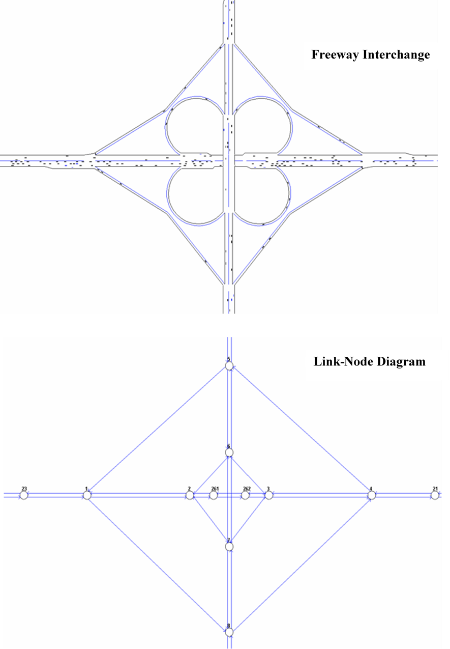

Table 8. Example node numbering convention

Segment	From Range	To Range	Description
0's	1	99	Miscellaneous
100's	100	199	Northbound Freeway Mainline
200's	200	299	Northbound Freeway Ramps
300's	300	399	Southbound Freeway Mainline
400's	400	499	Southbound Freeway Ramps
500's	500	599	Eastbound Freeway Mainline
600's	600	699	Eastbound Freeway Ramps
700's	700	799	Westbound Freeway Mainline
800's	800	899	Westbound Freeway Ramps
900's	900	999	Arterials

Link Geometry Data

The analyst should input the physical and operational characteristics of the links or the roadway segments into the model.

The analyst should model a study area that is of sufficient geographic scope to capture the impacts of the alternatives. The network modeled should not only include the area of interest but also facilities that feed demand into the study area and facilities that might potentially be the real cause of the bottleneck or congestion in the study area.

Some key geometric data that the analyst might need to input include:

• Number of lanes.
• Lane width.
• Link length.
• Grade.
• Curvature.
• Pavement conditions (dry, wet, etc.).
• Sight distance.
• Bus stop locations.
• Crosswalks and other pedestrian facilities.
• Bicycle lanes/paths.
• Others.

The specific data to be coded for the links will vary according to the microsimulation software. Use defaults if values are unknown for specific inputs (e.g., sight distance).

Traffic Control Data

Most microsimulation uses a time-step simulation to describe traffic operations (which is usually 1 s or less). Vehicles are moved according to car-following logic in response to traffic control devices and in response to other demands. Traffic control devices for microsimulation models will vary. Listed below are some examples:

• No control.
• Yield signs.
• Stop signs.
• Signals (fixed timed, actuated, adaptive).
• Ramp metering.
• Roundabouts.

Traffic Operations and Management Data

Traffic operations and management data for links consist of the following:

• Warning data (incidents, work zones, lane drops, exits, etc.).
• Regulatory data (speed limits, variable speed limits, high-occupancy vehicles (HOVs), high-occupancy toll (HOT), detours, lane channelization, lane use, truck restrictions, weight restrictions, etc.).
• Information (guidance) data (VMS).
• Surveillance detectors (type and location).

Traffic Demand Data

Traffic demand is defined as the number of vehicles and the percentage of vehicles of each type that wish to traverse the study area during the simulation time period.

Furthermore, it may be necessary to reflect the variation in demand throughout the simulation time period. In most software programs, the traffic entering into the network is usually defined by some parameter, and traffic leaving the network is usually computed based on parameters internal to the network (turning movements, etc.). The analyst should code the traffic volume by first starting from the external nodes (this is where the traffic is put into the model). Once all of the entering traffic volumes at the external nodes are coded, the analyst will then go into the model and define the turning movements and any other parameter related to route choice. The key traffic demand data are:

• Entry volumes by vehicle type and turning fractions at all intersections or junctions (random walk simulators).
• O-D/path-specific and vehicle data (path-specific simulators).
• Bus operations (routes and headways/schedules).
• Bicycle and pedestrian demand data.

Driver Behavior Data

Driver behavior is typically difficult to observe and collect. In addition, these data may change in response to non-normal conditions. At the base model development step, it is not critical to specify these inputs. Default values for driver behavior data are usually provided with the microsimulation software. Defaults will suffice if driver behavior data that reflects the local conditions do not exist. However, it is during the calibration step that these parameters will have to be adjusted carefully so that model represents the observed traffic conditions. For example, if the study area sees significant truck flow, distribution of driver types may be adjusted to capture the interactions between trucks and passenger cars. During alternatives analysis, if the driver behavior parameters have not been chosen carefully, you might get erroneous results that underestimate or overestimate the benefits and impacts.

Users may override the default values of any driver behavior parameters if valid observed data are available (e.g., desired free-flow speed, discharge headway, startup lost time at intersections, etc.). These deviations should be included in the Methods and Assumptions document. Some examples of driver behavior data that analyst can specify include:

• Driver's aggressiveness (for minimum headway in car-following, gap acceptance for lane changing, response to yellow interval).
• Availability of (real-time) information for the driver.
• Driver's compliance or response to information, such as traveler information, route guidance, advisory/regulatory speeds posted on VMS, HOV/HOT lane restrictions, etc.

Not all driver behavior data are observable in the field. When data are not observable, defaults may be used in the base model development stage. If a specific driver behavior is observable in the field, the analyst should collect them if resources permit before resorting to use of defaults.

Examples of observable driver behavior data include:

• Queue discharge and car-following headways.
• Gap acceptance.
• Start-up lost time.

Examples of unobservable driver behavior data include:

• Maximum speed and acceleration/deceleration rates.
• Lane change courtesy factor.
• Distribution of driver types (impacts aggressiveness).

Event Data

Event data are optional and will vary according to the specific application being developed by the analyst. Examples of event data inputs include:

• Blockages and incidents.
• Work zones.
• Parking activity in curb lane.

Some software allows the analyst to specify the location, time, and duration of the incident, the amount of rubbernecking, etc., while in others, incidents are not specified explicitly; rather these are modeled by specifying speed reduction zones. The analyst should refer the software's user guide for approaches to model events.

Simulation Run Control Data

All simulation software contains run control parameters to enable the analyst to customize the software operation for their specific modeling needs. These parameters will vary between software programs. They generally include:

• Length of simulation time.
• Selected MOEs or output (e.g., reports, animation files, or both).
• Resolution of simulation results (e.g., temporal and special resolution).
• Other system parameters to run the model.

The analyst should specify the length of the simulation time as the sum of the analysis period and the time needed for network loading, congestion build up, and congestion dissipation to capture demand and queuing accurately. If the analysis period is the AM peak period from 6 to 9 AM, we might have to specify a simulation period from 5 to 10 AM allowing for one hour for loading the network and congestion to build up, and one hour for congestion to dissipate. The additional time should be determined by examining the data.

Coding Techniques for Complex Situations

Microsimulation software allows the analyst to develop a model that represents the real-world situation. However, not all possible real-world situations were necessarily contemplated when the software was originally written. This is when the analyst, with a good understanding of the operation of the software, can "extend" the software to simulate conditions not originally incorporated into the microsimulation software. However, this should only be attempted after the tools, resources, and skills available are fully appreciated. This is because new tools continue to become available that account for selected real-world situations. These approaches should be discussed and agreed upon in the Methods and Assumptions document.

• A curb lane is heavily used for parking, loading, and unloading activities. As a result, this lane may be blocked virtually all the time. If the simulation software cannot correctly replicate the real situation, the analyst may consider removing this lane from the link. Alternately, the analyst may specify a speed reduction zone that extends the length of the loading zone, if the software has that capability, forcing vehicles to change lanes.
• Traffic regularly backs up on a freeway off-ramp, causing queuing on the freeway. However, instead of stopping on the freeway mainline lanes and blocking a lane, the queue forms on the shoulder of the freeway, keeping the right-hand lane open. If this is the case in the study area, the analyst may artificially extend the off-ramp length to realistically model the traffic in the field.

Example Problem: Base Model Development

Continuing with the Alligator City example problem from the previous chapters, the task is now to code the base model.

The first step is to code the link-node diagram. How this is best done can be determined from the software user's guide. Figure 7 shows the link-node diagram for the example problem. The next steps are to input:

• Link geometry data.
• Traffic control data for the Alligator City CBD (fixed-time control).
• Traffic operations and management data.
• Traffic demand data.
• Simulation run control data.

No driver behavior data have been collected for Alligator City and so, defaults are used.

Key Points

In summary, when developing the base model, the analyst should be aware that:

• Geographic scope of study area will impact the alternatives; so, broaden scope to look at roadway segments that feed the demand and roadway segments that may be the real bottleneck.
• Temporal scope of the simulation will impact the alternatives; so, broaden the scope to allow congestion to build up and dissipate.
• Base model should reflect the observed field geometry; so, overlay the model on a map of the area.
• Assumptions made should be documented so that results can be justified, and sensitivity analyses can be conducted, where applicable.