Traffic Analysis Toolbox Volume III: Guidelines for Applying Traffic Microsimulation Modeling Software 2019 Update to the 2004 Version
Chapter 4. Error Checking
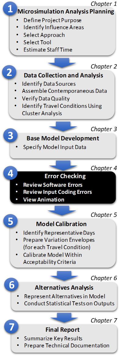
Figure 8. Diagram. Step 4: Error Checking
(Source: FHWA)
The error correction step is essential in developing a working model so that the calibration process does not result in parameters that are distorted to compensate for overlooked coding errors. This is Step 4 in the Microsimulation Analytical Process (Figure 8). The calibration process relies on the elimination of all major errors in demand and network coding before calibration.
Error checking involves various reviews of the coded network, coded demand, and default parameters. Error checking involves the following three stages:
- Review software errors.
- Review input coding errors.
- View animation to spot less obvious errors.
Review Software Errors
The analyst should review the software and user group web sites to ensure that he or she is aware of the latest known "bugs" and user workarounds for the software. The analyst should ensure that he or she is using the latest version and "patch" of the software, if any.
A checklist for verifying the accuracy of the coded input data is provided below:
Geometry:
- Check basic network connectivity (are all connections present?).
- Check link geometry (lengths, number of lanes, free-flow speed, facility type, etc.).
Control:
- Check intersection controls (control type, control data).
- Check for prohibited turns, lane closures, and lane restrictions at the intersections and on the links.
Demand:
- Check vehicle mix proportions at each entry node/gate/zone.
- Check identified sources and sinks (zones) for traffic.
- Verify zone volumes against traffic counts.
- Check vehicle occupancy distribution (if modeling HOVs).
- Check turn percentages (if appropriate).
- Check O-Ds of trips on the network.
Driver behavior and vehicle characteristics:
- Check and revise, as necessary, the default vehicle types and dimensions.
- Check and revise the default vehicle performance specifications.
The following techniques may be useful to increase the efficiency and effectiveness of the error-checking process:
- Overlay the coded network over a map of the study area to quickly verify the accuracy of the coded network geometry.
- If working with software that supports three-dimensional modeling, turn on the node numbers and look for superimposed numbers. They are an indication of unintentionally superimposed links and nodes. Two or more nodes placed in the same location will look like a single node when viewed in two dimensions. The links may connect to one of the nodes, but not to the other.
- For a large network, a report summarizing the link attributes should be created so that their values can be easily reviewed.
- Use color codes to identify links by the specific attribute being checked (e.g., links might be color-coded by free-flow speed range). Out-of-range attributes can be identified quickly if given a particular color. Breaks in continuity can also be spotted quickly (e.g., a series of 56-km/h (35-mi/h) links with one link coded as 40 km/h (25 mi/h)).
View Animation
Animation output enables the analyst to see the vehicle behavior that is being modeled and assess the reasonableness of the microsimulation model itself. Running the simulation model and reviewing the animation, even with artificial demands, can be useful to identify input coding errors. The analyst inputs a very low level of demand and then follows individual vehicles through the network. Aberrant vehicle behavior (such as unexpected braking or stops) is a quick indicator of possible coding errors. At this stage, the analyst is not required to perform multiple runs of the model by changing the random number seeds; a single random-number-seed run will suffice.
A two-stage process can be followed in reviewing the animation output. Run the animation at an extremely low demand level (so low that there is no congestion). The analyst should then trace single vehicles through the network and see where they unexpectedly slow down. These will usually be locations of minor network coding errors that disturb the movement of vehicles over the link or through the node. This test should be repeated for several different O-D zone pairs.
Once the extremely low demand level tests have been completed, then run the simulation at 50 percent of the existing demand level. At this level, demand is usually not yet high enough to cause congestion. If congestion appears, it may be the result of some more subtle coding errors that affect the distribution of vehicles across lanes or their headways. Check entry and exit link flows to verify that all demands are being correctly loaded and moved through the network.
The animation should be observed in close detail at key bottleneck areas to determine if the animated vehicle behavior is realistic. If the observed vehicle behavior appears to be unrealistic, the analyst should explore the following potential causes of the unrealistic animation in the order shown below:
- Error in Analyst's Expectations: The analyst should first verify in the field the correct vehicle behavior for the location and time period being simulated before deciding that the animation is showing unrealistic vehicle behavior. Many times, the analyst's expectations of realistic vehicle behavior are not matched by actual behavior in the field. Analysts should not expect classic macroscopic traffic-flow concepts to apply at the microscopic individual-vehicle level. Macroscopic flow concepts (e.g., no variance in mean speed at low flow rates) do not apply to the behavior of an individual vehicle over the length of the highway. An individual vehicle's speed may vary over the length of the highway and between vehicles, even at low flow rates. Macroscopic flow theory refers to the average speed of all vehicles being relatively constant at low flow rates, not individual vehicles. Field inspection may also reveal the causes of vehicle behavior that are not apparent when coding the network from plans and maps. These causes need to be coded into the model if the model is expected to produce realistic behavior. Transportation Management Centers (TMC) with high-density camera spacing will be very helpful in reviewing the working model. Many TMCs are now providing workstations for traffic analysis/simulation staff.
- Error in Analyst's Data Coding: The analyst should check for data coding errors that may be causing the simulation model to represent travel behavior incorrectly. Subtle data coding errors are the most frequent cause of unrealistic vehicle behavior in commercial microsimulation models that have already been subjected to extensive validation. Subtle coding errors include apparently correctly coded input that is incorrect because of how it is used in the model to determine vehicle behavior. For example, it could be that the warning sign for an upcoming off-ramp is posted in the real world 0.40 km (0.25 mi) before the off-ramp; however, because the model uses warning signs to identify where people start positioning themselves for the exit ramps, the analyst may have to code the warning sign at a different location (the location where field observations indicate that the majority of the drivers start positioning themselves for the off-ramp).
A comparison of model animation to field design and operations is highly essential. Some of the things to look for include:
- Overlooked data values that require refinement.
- Aberrant vehicle operations (e.g., drivers using shoulders as turning or travel lanes, etc.).
- Previously unidentified points of major ingress or egress (these might be modeled as an intersecting street).
- Operations that the model cannot explicitly replicate (certain operations in certain tools/models), such as a two-way center turn lane (this might be modeled as an alternating short turn bay).
- Unusual parking configurations, such as median parking (this might be modeled operationally by reducing the free-flow speed to account for this friction).
- Average travel speeds that exceed posted or legal speeds (use the observed average speed in the calibration process).
- Turn bays that cannot be fully utilized because of being blocked by through traffic.
- In general, localized problems that can result in a system wide impact.
Residual Errors
If the analyst has field-verified his or her expectations of traffic performance and has exhausted all possible input errors, and the simulation still does not perform to the analyst's satisfaction, there are still a few possibilities. The desired performance may be beyond the capabilities of the software, or there may be a software error.
Software limitations can be identified through careful review of the software documentation. If software limitations are a problem, the analyst might seek an alternate software program without the limitations. Advanced analysts can also write their own software interface with the microsimulation software (called an "application program interface" (API)) to overcome the limitations and produce the desired performance. Any changes made to override the simulation software's capabilities should be documented in the Methods and Assumptions document.
Software errors can be tested by coding simple test problems (such as a single link or intersection) where the result (such as capacity or mean speed) can be computed manually and compared to the model. Software errors can only be resolved by working with the tool developer.
Key Decision Point
The completion of error checking is a key decision point. The next task-model calibration-can be very time-consuming. Before embarking upon this task, the analyst should confirm that error checking has been completed, specifically:
- All input data are correct.
- Values of all initial parameters and default parameters are reasonable.
- Animated results look fine based on judgment or field inspection.
Once the error checking has been completed, the analyst has a working model (though it is still not calibrated).
Example Problem: Error Checking
Continuing with the Alligator City problem from the previous chapters, the task is now to error check the coded base model.
Software: The latest version of the software was used. Review of the model documentation and other material in the software and user groups' web sites indicated that there were no known problems or bugs related to the network under study and the scenarios to be simulated.
Review of Input Data and Parameters: The coded input data were verified using the input files, the input data portion of the output files, static displays, and animation.
First, the basic network connectivity was checked, including its consistency with coded geometry and turning restrictions. All identified errors were corrected. For example, there was a fatal error that one of the SB Riverside Parkway links didn't exist. It was found that the link number had a typographical error.
Static network displays were used extensively to verify the number of lanes, lane use, lane alignment (i.e., lane number that feeds the downstream through link), and the location of lane drops. At this step, the consistency of link attributes was checked. For example, is the free-flow speed of ~90 km/h (55 mi/h) coded for all freeway links?
Next, the traffic demand data were checked. Input volumes at the network entrances were specified in four time slices. The input values were checked against the collected data.
Traffic signals coded at each intersection were reviewed. For fixed-time signals, the phasing and signal settings were checked. There was a fatal error that indicated Phase 1 at one of the intersections in Downtown Alligator City was incorrect. Phase 1 was defined as left-turns from the E-W street. But the cross street (N-S street) was coded as one-way. So, left turns are not allowed from the eastbound street. This was fixed.
Special attention was given to the traffic patterns at the interchange ramp terminals to avoid unrealistic movement. The software provisions (and options) were exercised to force the model not to assign movements to travel paths that were not feasible.
Vehicle characteristics were reviewed.
Review Animation: Following the checking of the input data, the model was run using very low demand volumes to verify that all of the vehicles travel the network without slowdowns. This step uncovered minor errors in the link alignments that needed adjusting.
Next, the traffic demands were specified to about 50 percent of the actual volumes and the simulation model was rerun. Animation was used to verify that all demands were properly loaded in the network links and the traffic signals were properly operating. The link and system performance measures (travel time, delay) were also checked for reasonableness (i.e., they should reflect free-flow conditions).
Careful checking of the animation revealed subtle coding problems. For example, the coded distance of a warning sign for exiting vehicles from the Victory Island Bridge affected the proper simulation of driver behavior. These problems were corrected.
Key Decision Point: The model, as revised throughout the error-checking process, was run with all the input data (actual demands) and the default model parameters. The output and animation were also reviewed and discussed with the Alligator City agency staff who were familiar with the study area. The conclusion was that the model is working properly.
Key Points
In summary, when checking errors, the analyst should:
- Use structured/consistent processes.
- Check for "known" bugs and follow recommendations of the developer.
- Use graphical display and animation in the debugging process.
- Conduct an independent review to improve model quality.