Traffic Analysis Toolbox Volume III: Guidelines for Applying Traffic Microsimulation Modeling Software 2019 Update to the 2004 Version

Chapter 6. Alternatives Analysis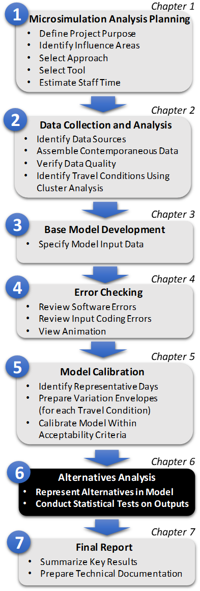

Project alternatives analysis is Step 6 in the Microsimulation Analytical Process (Figure 13). It is the reason for developing and calibrating the microsimulation model. The lengthy model development process has been completed and now it is time to put the model to work. If the alternatives are to be evaluated in target future year, a future travel demand forecast will have to be incorporated to create future year model variant for each travel condition. The analyst should also create model sub-variants for each competing alternative for each travel condition. Alternatives analysis requires comparison between simulation runs that may have similar results. In these cases, there should be consideration of the impact of model variation. Even small variation resulting from simulation model stochasticity may impact the statistical validity observed in simulation outputs, which will in turn impact investment decisions. Hence, the analyst should consider multiple runs by varying random number seeds for alternatives analysis. As a first step, the analyst should run each model sub-variant four times under different random number seeds to assess variability in tactical driver behavior in the model sub-variant. Randomness in simulation outputs are analyzed to determine the required number of runs to satisfactorily assess statistical validity when comparing the impacts of competing alternatives. The analyst then runs each model sub-variant the required number of replication for each alternative to generate the necessary output to generate the key performance measures. A statistical test is then conducted to determine whether any differences between two alternatives are statistically significant, that is, these differences meet the minimum criteria that bounds the risk that differences are only related to randomness in model outputs.

Forecast Future Demands

Some analyses require the explicit consideration of system performance in future years. In these cases, the analyst should make a forecast of future year travel demand. Forecasts of future travel demand significantly different from current conditions are best obtained from a travel demand model, or from a multi-resolution modeling approach where the full range of dynamic travel demand attributes (including trip generation, distribution, mode choice, and trip start timing) can be considered collectively from the perspective of the complete transportation system.

These models require a great deal of effort and time to develop and calibrate. If one does not already exist, then the analyst (in conjunction with the simulation project management) may opt to develop demand forecasts based on historic growth rates. A trend-line forecast might be made, assuming that the recent percentage of growth in traffic will continue in the future. These trend-line forecasts are most reliable for relatively short periods of time (5 years or less). They do not take into account the potential of future capacity constraints to restrict the growth of future demand. Additional information and background regarding the development of traffic data for use in highway planning and design may be found in other resources (For example, the National Cooperative Highway Research Program (NCHRP) Report 765). Whatever the method selected, a description of the approach (and the rationale for the approach) should be captured within the Methods and Assumptions document.

Regardless of which method is used to estimate future demand (explicit travel demand modeling or simple trend line), care should be taken to ensure that the forecasts are a reasonable estimate of the actual amount of traffic that can arrive within the analytical period at the study area. Regional model forecasts are usually not well constrained to system capacity and trend-line forecasts are totally unconstrained. MRM approaches are generally more appropriate for future year demand estimation when travel demand is significantly larger than current travel demand.

All forecasts are subject to uncertainty. It is risky to assess competing alternatives to a precise future condition given the uncertainties in the forecasts. There are uncertainties in both the probable growth in demand and the available capacity that might be present in the future. Slight changes in the timing or design of planned or proposed capacity improvements outside of the study area can significantly change the amount of traffic delivered to the study area during the analytical period. Changes in future vehicle mix and the timing of travel demand can have a significant impact. Similarly, changes in economic development and public agency approvals of new development can significantly change the amount of future demand. Thus, it is good practice to plan for a certain amount of uncertainty explicitly in the analysis. This level of uncertainty is the purpose of sensitivity testing (explained in a separate section below).

Represent Alternatives

In Step 1, competing alternatives are identified and detailed. Often times, however, the specificity required by the microsimulation to represent these alternatives is not evident until the travel conditions are defined. In this regard, the analyst can play a key role in working with stakeholders to further develop the concept in each alternative. For example, when considering a specific representative day with an incident, stakeholders may have to collectively make a decision as to whether this particular incident would trigger a response from the incident management system.

Detailed guidance on the accurate representation of elements of alternatives is highly dependent on the tool selected and is not in scope for this guidebook. However, several federal reports may be useful resources for specific types of alternatives. For example, TAT Volume XII is used for work zone alternatives, and TAT Volume XIII is used for integrated corridor alternatives. Both guides can be obtained from https://ops.fhwa.dot.gov/trafficanalysistools/.

Determine Required Number of Replications

Microsimulation models rely on random numbers to provide non-uniform elements of tactical driver behavior. These elements may include the type and sequencing of vehicles generated at origins, tactical decisions made regarding route and gap acceptance, and aggressiveness in lane changing behavior. The cluster analysis and calibration to specific travel conditions performed in the previous steps isolate the first order determinates of system variation (changes in travel demand patterns, incident patterns, and weather conditions). The inherent randomness in microsimulation models related to tactical driver behavior is second order compared to travel conditions. However, randomness from these stochastic processes within a microsimulation should still be accounted for within the alternatives analysis.

To generate an initial assessment of the impact of this randomness in support of alternatives analysis, run the model sub-variant associated with each alternative and travel condition four times using different random seeds. How random seeds are implemented in each simulation tool varies, but randomness is generally included in a default set of tactical driver behavioral models and vehicle generation processes. The minimum number of replications is calculated using the following equation:

\(N_{\min} = \left( \frac{t_{n - 1,\ 95\%}s}{e\overline{x}} \right)^{2}\)(15)

where:

\(N_{\min}\) : Required number of model runs

n : Number of initial model runs (i.e., 4)

\(\overline{x},\) \(s\) : Mean and standard deviation of the initial runs

\(t_{n - 1,95\%}\) : t statistic for n-1 degrees of freedom and 95% confidence level

e : Tolerance error

A confidence level of 95% is a traditional default to use. However, it may not always be the best value for every analysis. We need to identify an appropriate confidence level (a measure of accuracy when differentiating samples) and tolerance error (a measure of observed data precision).

Confidence Level should be determined by the decision-maker and not the analyst, prior to alternatives analysis. The choice of confidence level is typically associated with the required certainty for the decision-maker. In a broad sense, a higher confidence level is chosen when the consequences of being wrong are significant. For example, when analyzing safety critical systems, like airplane engine failures, the required confidence level might be 99.99%. However, the assessment of transportation alternatives may not be in the same category of down-side risk. Typical values are set between 80-95%, with 95% representing the highest confidence. A 95% confidence level is assumed unless otherwise set by project management (e.g., local agency policy) and logged in the Methods and Assumptions document.

Tolerance error, e, is calculated individually for each observed time-variant measure based on the two critical time periods, \(t_{1}\) and \(t_{2}\), identified for that measure. The expectation is that the most within-cluster variation is reflected at the critical time periods, when the dynamics of the system are in flux, transitioning from rise-to-fall (for travel time) or fall-to-rise (for throughput).

First, construct the confidence interval as follows:

\(\overline{x} \pm \left\{ t_{n - 1,95\%}\left( \frac{s}{\sqrt{n}} \right) \right\}\)(16)

where:

\(\overline{x},s\) : Mean and standard deviation

n : Number of observations

\(t_{n - 1,\ \ 95\%}\) : t statistic for n-1 degrees of freedom and 95% confidence level

Tolerance error is computed as follows:

\(e = \ \frac{t_{n - 1,95\%}\left( \frac{s}{\sqrt{n}} \right)}{\overline{x}}\)(17)

The numerator is also known as the margin of error.

Let \({\overline{x}}_{1}\), \(s_{1}\)and \({\overline{x}}_{2}\), \(s_{2}\) be the mean and standard deviation of the measure at the two critical time periods for a given cluster, with \(\text{n\ }\)observations (or days). Calculate the tolerance error for the measure at the two critical time periods using the equations:

\(e_{1} = \frac{t_{n - 1,95\%}\left( \frac{s_{1}}{\sqrt{n}} \right)}{{\overline{x}}_{1}}\)(18)

\(e_{2} = \frac{t_{n - 1,95\%}\left( \frac{s_{2}}{\sqrt{n}} \right)}{{\overline{x}}_{2}}\)(19)

Set the tolerance error as the maximum of the two calculated tolerance errors at the two critical time intervals.

Run the model 4 times and compute the simulated average \(\overline{x}\) and standard deviation \(s\) of the critical time-variant measures. Let \(t_{3,\ 95\%}\) be the t-statistic associated with a 95% confidence level and three degrees of freedom (3.182).

The required number of runs is calculated using the following formula, rounded up to the nearest whole number:

\(N_{\min} = \left( \frac{t_{3,95\%}s}{e\overline{x}} \right)^{2}\)(20)

The steps should be repeated for all key measures of interest and all clusters, and corresponding minimum number of runs should be calculated. The minimum number of model replications is then taken as the maximum of the minimum number of runs (\(N_{\min}\)) computed for all key measures and all clusters.

In less congested conditions, there may be very little day to day variation resulting in very small tolerance errors. This can be problematic from a computational perspective since a small tolerance error will result in a large \(N_{\min}\) with no gain in analytical insight as the result is many repetitions of essentially fixed near free-flow conditions. To guard against unreasonable \(N_{\min}\) driven by small observed variation, we enforce a minimum floor for tolerance error of 5% as a practical guideline.

Test Differences in Alternatives Performance

When the microsimulation model is run several times for each alternative, the analyst may find that the variance in the results for each alternative is close to the difference in the mean results for each alternative. How is the analyst to determine if the alternatives are significantly different? To what degree of confidence can the analyst claim that the observed differences in the simulation results are caused by the differences in the alternatives and not just the result of using different random number seeds? This is the purpose of statistical hypothesis testing.

Perform Hypothesis Testing

In this step, we compare the results obtained examining two alternatives to see if the differences are statistically significant.

First, calculate the average performance measures for the two alternatives, \(x_{1}\) and \(x_{2}\), reflecting the frequency of each travel condition. For simpler measures like delay, this is a simple weighted sum using the frequency of each travel condition, as shown below:

\({\overline{x}}_{j} = \frac{\sum_{i = 1}^{C}\left( x_{i} \times n_{i} \right)}{\sum_{}^{}n_{i}}\)(21)

where:

\({\overline{x}}_{j}\) : Weighted average of measure for alternative j

i : Cluster ID

C : Total number of clusters

\(x_{i}\) : Average performance measure estimate across all random number runs (i.e., \(N_{\min}\)) for Cluster i

n_i : Number of days in Cluster i

For other measures, like reliability, the individual results are combined in order to identify percentile-based statistics, such as 95^th percentile planning time index.

Next, calculate the sample variance for the two alternatives as follows:

\(s_{j}^{2} =\) \(\frac{\sum_{i = 1}^{C}\left( x_{i} - {\overline{x}}_{j} \right)^{2}}{C}\)(22)

where:

\(s_{j}^{2}\) : Variance of measure for alternative j

We assume population variances are unknown and equal. If variances are not equal, then Welch's t-test should be used. \(n_{1}\) and \(n_{2}\) are the number of simulation runs for the two alternatives. The pooled variance \(s_{p}^{2}\) is the weighted average of the two sample variances, \(s_{1}^{2}\) and \(s_{2}^{2}\):

\(s_{p}^{2} = \frac{\left( n_{1} - 1 \right)s_{1}^{2} + \left( n_{2} - 1 \right)s_{2}^{2}}{\left( n_{1} + n_{2} - 2 \right)}\)(23)

Set up the hypotheses based on the evidence from the sample:

• Null Hypothesis, H₀: \(\mu_{1} \geq \mu_{2}\) OR \(\mu_{1} \leq \mu_{2}\)
• Alternate Hypothesis, H_A: \(\mu_{1} < \mu_{2}\) OR \(\mu_{1} > \mu_{2}\)

Calculate the test statistic:

\(t_{\text{calculated}} = \ \frac{\left( {\overline{x}}_{1} - {\overline{x}}_{2} \right)}{\sqrt{s_{p}^{2}\left( \frac{1}{n_{1}} + \frac{1}{n_{2}} \right)}}\)(24)

Perform the hypothesis test:

• For H₀: \(\mu_{1} \geq \mu_{2}\), if \(t_{\text{calculated}} \leq t_{n_{1} + n_{2} - 2,\ 95\%}\), reject H₀ and accept H_A. Otherwise, we do not have enough evidence to reject H_0.
• For H₀: \(\mu_{1} \leq \mu_{2}\), if \(t_{\text{calculated}} \geq t_{n_{1} + n_{2} - 2,\ 95\%}\), reject H₀ and accept H_A. Otherwise, we do not have enough evidence to reject H_0.

Perform Sensitivity Testing

A sensitivity analysis is a targeted assessment of the reliability of the microsimulation results, given the uncertainty in the input or assumptions. The analyst identifies certain input or assumptions about which there is some uncertainty and varies them to see what their impact might be on the microsimulation results.

Additional model runs are made with changes in demand levels and key parameters to determine the robustness of the conclusions from the alternatives analysis. A sensitivity analysis of different demand levels is particularly valuable when evaluating future conditions. Demand forecasts are generally less precise than the ability of the microsimulation model to predict their impact on traffic operations. Additional runs may also be needed to address sensitivity to assumptions made in the analysis where the analyst may have little information, such as the percent of drivers listening to specific traveler information services.

Example Problem: Alternative Analysis

For the Alligator City travel time example, we examine the average and standard deviation of travel times at our two critical time periods, 7:15 AM and 7:45 AM. At 7:15 AM, the average travel time is 32.6 minutes, and the standard deviation is 2.2 minutes. At 7:45 AM, the average travel time is 31.0 minutes, and the standard deviation is 1.7 minutes. Raw tolerance error (excluding the 5% floor) at 7:15 AM is 0.97% and 0.81% at 7:45 AM. Since this falls below the 5% floor on tolerance error, a tolerance error of 5% is used.

Running the model variant 4 times for this condition produces an average travel time of 32.7 minutes with a standard deviation of 1.46 minutes. In this case the minimum number of runs is \({(\frac{3.182 \times 1.46}{0.05 \times 32.7})}^{2} = 8.07\) runs. For this particular measure, alternative, and travel condition, 9 runs are required (8.07 rounded up to the nearest whole number).

A note regarding large N. In some cases where a model is not stable, a very large value of N (>20) may result. In these cases, it is not recommended to replicate 20 or more runs of the model sub-variant, but rather to investigate the reasons why a particular model sub-variant produces such a large variation in outputs. Sometimes it is an indicator that unrealistic gridlock conditions are being generated within the model, the results of which can skew model outputs. Model instability can also be symptomatic of model coding errors.

Table 13 provides a summary of aggregate statistics for the two competing Alligator City alternatives and a Do-Nothing case after a uniform number of random number seeds has been conducted (in this case, 5). Travel time is an aggregated value over the two major routes considering all time periods in the morning peak and weighted by each of the travel conditions. Throughput is a measure of average vehicles per hour exiting of all bridge and tunnel exits into Alligator City, considering all time periods in the morning peak period and weighted by travel condition. Planning time index is calculated as an origin-destination level measure from West Hills to Alligator City considering both potential routes and the variation in travel time over all time periods it the morning peak. The planning time index represents the ratio of the 95^th percentile travel time to free-flow (uncongested) travel time from West Hills to Alligator City considering all travel conditions.

Table 13. Aggregate Results from Alligator City Alternative Analysis

Alternative	Performance Measures
	Travel Time		Throughput		Plan Time Index
	Average	Std. Dev.	Average	Std. Dev.	Average	Std. Dev.
Current Baseline	17.1	0.3	7463	189	2.02	0.25
Do Nothing	19.5	0.6	7209	369	2.15	0.35
Better Bridge and Tunnel	16.4	0.6	8337	450	2.65	0.36
Adapt and Redirect	16.6	0.8	8199	210	1.85	0.25

Examine a hypothesis considering the planning time index value for Adapt and Redirect (Alternative 1) compared to Better Bridge and Tunnel (Alternative 2). In this case, we seek to test whether the lower value for Adapt and Redirect when compared to that for Better Bridge and Tunnel is statistically significant. The hypotheses are set as follows: H₀: \(\mu_{1} \geq \mu_{2}\), H_A: \(\mu_{1} < \mu_{2}\).

The estimate for the pooled variance is:

\[s_{p}^{2} = \frac{8 \times {0.36}^{2} + 8 \times {0.25}^{2}}{9 + 9 - 2} = 0.096\]

\[t_{\text{calculated}} = \frac{1.85 - 2.65}{\sqrt{0.096 \times (\frac{1}{9} + \frac{1}{9})}} = - 5.48\]

\(t_{\text{calculated}} < \ t_{16,\ 95\%}\ \) (-5.48 < 1.746), so we reject the null hypothesis that the planning time index for Alternative 1 is greater than or equal to that for Alternative 2, and conclude that the planning time index for Alternative 1 is statistically smaller. Similar comparisons of travel time and throughput can also be made. The overall result is that while the Adapt and Redirect (Alternative 1) generates a lower planning time index (i.e., higher reliability), for other measures the alternative is not clearly better (and for throughput worse). Similar comparisons should be made for the remaining alternatives.

Key Points

In summary, when conducting alternatives analysis:

• Forecasting major shifts in future travel demand should be analyzed separately from the microsimulation.
• Every alternatives analysis requires multiple runs with different random seeds.
• Randomness in simulation outputs are related to variations in driver behavior models.
• Variation in results from different random seeds are not indicative of first order system variation, which are determined by travel conditions.
• Ensure models are stable and do not create unrealistic gridlock conditions, as this will create artificial (and dramatic) variation in outputs.