Traffic Analysis Toolbox Volume III: Guidelines for Applying Traffic Microsimulation Modeling Software 2019 Update to the 2004 VersionAppendix A. Work Zone Case Study in the Seattle I-405 CorridorAppendix A presents a hypothetical case study in a large and realistic urban corridor to illustrate the updated 2019 guidelines of traffic microsimulation. In this case, the analytical project regards the application of a microsimulation analysis to support cost-effective planning for a significant work zone project. This case study was conducted using Washington State Department of Transportation (WSDOT) and University of Washington data archives and an existing WSDOT microsimulation model. However, the hypothetical situation described in this study (work zone repair in response to sinkhole damage from seismic activity) is neither based on actual events, nor do the alternatives analyzed here reflect WSDOT policies or contingency planning. The Seattle I-405 Corridor I-405 Corridor is a major commuter corridor in the Seattle area subject to periods of high travel demand and resultant congestion. In addition, the corridor experiences significant travel time variability as a result of dynamic incident patterns and frequent rain and fog. Figure 15 depicts the geographical coverage of the I-405 corridor in this case study, extending from a junction north of Lake Washington with I-5 to a junction rejoining I-5 south of Lake Washington. The length of the I-405 corridor is 29.5 miles. 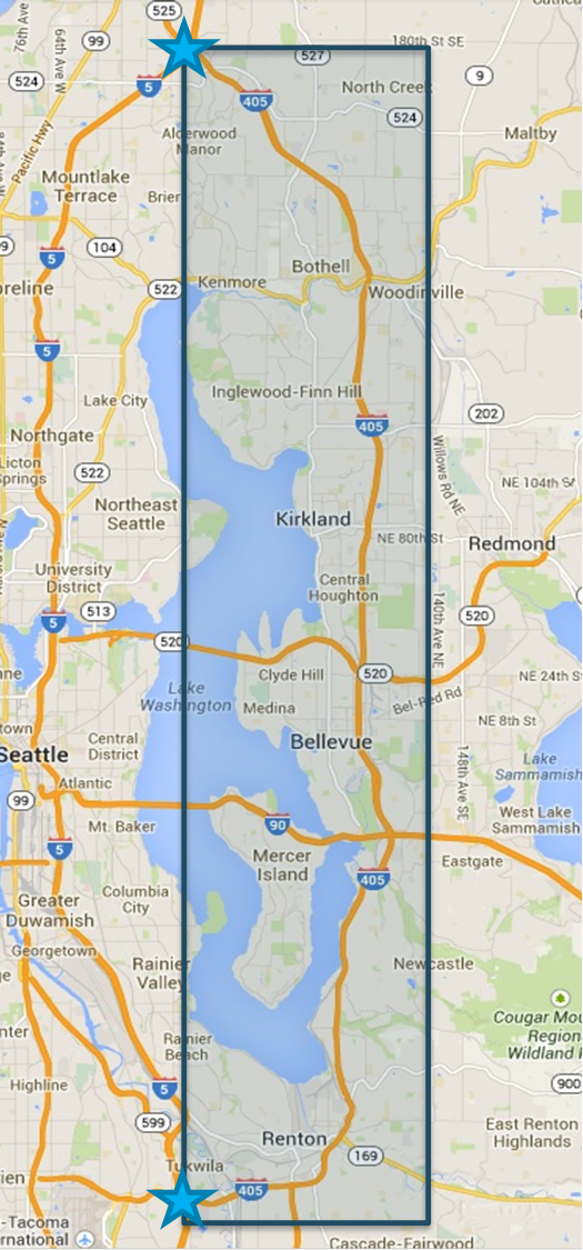
Figure 15. Map. I-405 Geographical Coverage Purpose, Approach and Tool In this hypothetical case study, the product of unanticipated seismic activity in the region has resulted in significant damage to the I-405 freeway facility. Two sinkholes have damaged segments of the I-405 roadway. The road is still passable and usable in all segments. However, significant rehabilitation is required within six months to the damaged sections. If these issues are not addressed within six months, there are risks of more substantial structural damage and the need for more expensive and complicated reconstruction. Repair work can and will be done on all available nights, weekends, and weekday midday periods. As a general policy, no work is planned for AM (6-10 AM) or PM peak (3-7 PM) periods because of expected congestion. However, completing the needed repair in six months with no peak period work will require expensive, expedited night and weekend work. Because of these high costs, there is interest in determining if some targeted peak period lane closures might be considered in this case to complete the work in the six-month window without incurring the additional expense of expedited off-peak work. In order to inform this decision, alternatives analysis using microsimulation is selected for the project given a need for lane-level assessment of the precise alternative timing of potential lane closures. Total additional delays caused by a work zone is used as the primary measure differentiating alternatives, and travel time reliability is used as a supplemental measure of effectiveness. Two alternatives are proposed regarding the work zone schedule:
Available Data The Washington Department of Transportation (WSDOT) regularly utilizes advanced data and simulation analytics to improve investments for operations. The agency has extensive experience in collecting traffic data, building and calibrating simulation models, and measuring system performance. At FHWA request, WSDOT provided 2012 traffic data, travel time information, incident data and weather information listed below. Data quality was checked/verified utilizing web-based capabilities provided by University of Washington.
As shown in Figure 16, two bottleneck locations were identified based on WSDOT Traffic Map Archive (http://www.wsdot.wa.gov/data/tools/traffic/maps/archive/?MapName=SysVert) and speed data. Note that these recurrent bottlenecks are characterized using the observed 2012 corridor data, and do not reflect the presence of the hypothetical sinkhole-related work zones. 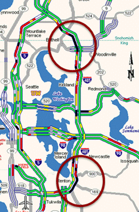
Figure 16. Map. Bottleneck Locations
Cluster Analysis This case study focuses on both northbound (NB) and southbound (SB) directions on the weekday morning peak, which is from 6:00 AM to 10:00 AM. Note that NB and SB facilities are analyzed together (not separately) in a single analysis. After removing weekends and holidays (not germane to our alternatives analysis), and the days where contemporaneous data were not available, a total of 196 weekdays were identified for cluster analysis. WEKA (Waikato Environment for Knowledge Analysis) is used in this case study for data normalization and analysis. The steps listed in Chapter 2 to identify travel conditions were followed and results obtained using the 196-day data archive, reported below. Steps 1 - 4: Identify and Select Attributes More than 30 potential attributes were initially considered for analysis. The following ten attributes were identified for each of the 196 days to represent variation in travel demand, underlying incident and weather-related impacts, and resulting aspects of system performance:
Since the selected attributes are numeric data, no further data processing is required. WEKA provides an automatic normalization function during cluster analysis process, so in this case study, data will be normalized through WEKA. Steps 5 - 6: Perform Clustering and Identify Stopping Criterion The WEKA K-Means option was used to perform cluster analysis. First, we calculated the maximum number of clusters to consider, \(2\sqrt{n/2} = 2\sqrt{196/2} = 19.8\). Therefore, the maximum cluster size we considered was set to 20. For the evaluation of the suitability of the WEKA-identified clusters by number of clusters, we first selected Option 2 (see Equation 3 of Chapter 2), heuristic assessment. Figure 17 plots the heuristic fitness index against the clusters obtained under a constraint of four clusters through 20 clusters. As a reminder, the heuristic index is obtained by multiplying the number of clusters by the average coefficient of variation among identified clusters. A cluster size of three was also considered but the obtained heuristic fitness value was too large to be included in this Figure 17. A five-cluster grouping generates the lowest heuristic index. 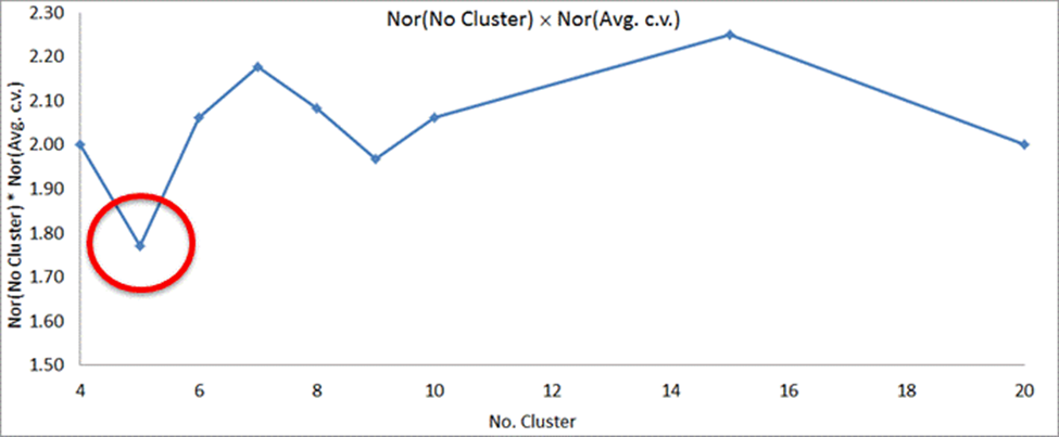
Figure 17. Chart. Plot of Heuristic Index Calculation Results For this study, we also examined the Sum of Squared Error (SSE), as another indicator of cluster performance. SSE is a measure of intra-cluster variation, essentially providing a measure of how close each of the days in the cluster are to the mean value for the ten critical attributes. Table 14 and Table 15 present a comparison of the SSE for 4-cluster, 5-cluster and 6-cluster cases. In Table 14, the 5-cluster case has a lower average coefficient of variation and the 6-cluster case has the lowest SSE. In Table 15, the 5-cluster case has a high SSE in the Cluster 4 group, which indicates that there are potentially a large number of different days in this larger cluster. Adding one more cluster (i.e., the 6-cluster case) lowers the SSE significantly for this group. Therefore, a 6-cluster case is chosen for this case study.
After running WEKA using the K-Mean approach with the number of clusters as six, Table 16 summarizes the cluster analysis results. As shown in Table 16, each cluster (or travel condition) is given a descriptive name based on the values of the attributes. Figure 18 is the travel condition dartboard, which provides a graphical view of the six identified travel conditions. 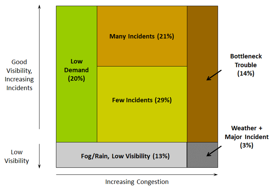
Figure 18. Diagram. I-405 Travel Condition Dartboard Model Calibration WSDOT provided an I-405 VISSIM [26] model previously calibrated for a "nominal average day" for the purposes of an earlier study. This network is used as the initial working base model to perform calibration for the six identified travel conditions. In this model, calibration process, travel time and bottleneck throughout are selected as the key performance measures. Step 1: Identify Representative Days Based on the guidance in Chapter 5, a single representative day for each travel condition is selected that minimizes the average Euclidean distance. Figure 19 depicts the travel time and bottleneck throughput profiles of all the clusters compared to the "nominal average day" for both NB and SB directions. From the figures, one may observe that the profiles of the six travel conditions are different from each other and the "nominal average day" only has a good match for the Few Incidents travel condition (Cluster 5). 
Figure 19. Chart. Travel Time and Bottleneck Throughput Profiles for Each Travel Condition Steps 2-3: Prepare Variation Envelopes and Calibrate Model Variants 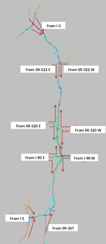
Figure 20. Map. Locations for Demand Adjustment In this case study, corridor travel time and bottleneck throughput at 15-min. time intervals are selected as calibration performance measures. The selection of the two bottleneck locations is described previously. The variation envelopes for all the travel conditions are created based on the guidance in Chapter 5. Figure 20 shows a subset of travel demand origins that were the focus of demand adjustment (both total flow and temporal profile) during the calibration process. The AM peak period extends from 6:00 AM to 10:00 AM. The simulation is set to start at 5:30 AM to provide a 30-min. warm up time and end at 10:30 AM to make sure the vehicles starting at 10:00 AM can complete the trip and be included into calculation. It is noteworthy that the 5-hour (5:30 to 10:30 am) simulation running time is about 3 hours of actual time. In this case study, demand, speed distribution, and car-following headways are used as adjustable parameters. Figure 21 through Figure 26 illustrate the variation envelopes and calibration results for each travel condition. In each figure, the orange line represents the selected representative day, the pink and light green dashed lines are the 1 sigma and ~2 sigma bands, and the green triangles are the simulation results. The two critical time intervals are selected based on the guidance listed in Chapter 5. The critical time intervals for travel time are marked with red dots along the representative day line. The critical time intervals for bottleneck throughput are indicated with red circles. Table 17 summarizes the calculation results of the acceptability criteria listed in Chapter 5. 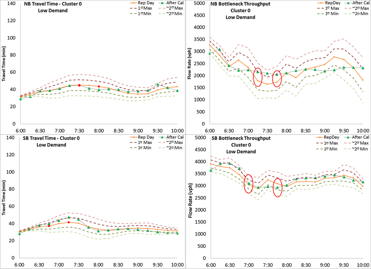
Figure 21. Chart. Variation Envelope and Calibration Results for Low Demand Travel Condition 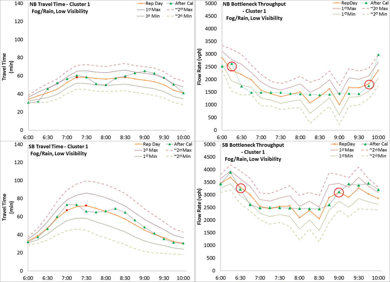
Figure 22. Chart. Variation Envelope and Calibration Results for Low Visibility Travel Condition 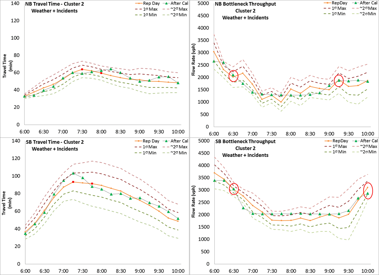
Figure 23. Chart. Variation Envelope and Calibration Results for Weather + Incidents Travel Condition 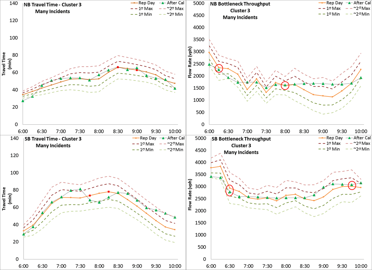
Figure 24. Chart. Variation Envelope and Calibration Results for Many Incidents Travel Condition 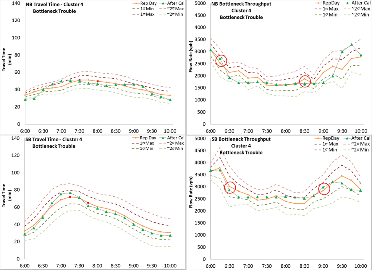
Figure 25. Chart. Variation Envelope and Calibration Results for Bottleneck Trouble Travel Condition 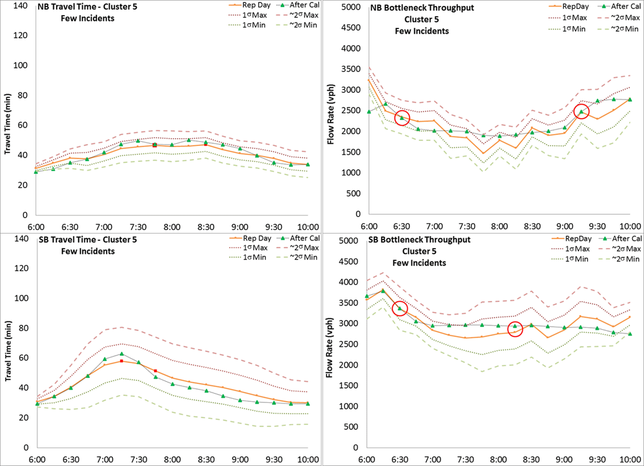
Figure 26. Chart. Variation Envelope and Calibration Results for Few Incidents Travel Condition (Source: FHWA) Table 17. Summary of Acceptability Criteria Calculation Results 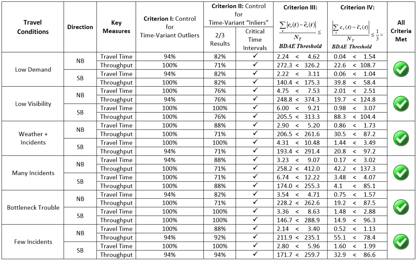
As noted in the guidance in Chapter 5, since only 17 time intervals are used to characterize time-dynamics in this case study, one simulated result is allowed to fall outside the ~2 Sigma Band for Criterion I. Therefore, in Table 17, 94% still meets Criterion I. The simulation models for all the identified travel conditions are now well-calibrated for work zone alternatives analysis. Work Zone Alternative Analysis 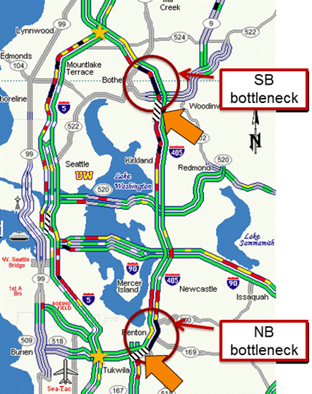
Figure 27. Map. Sinkhole Damaged Sections When modeling hypothetical active and inactive work zone conditions, several assumptions were made and logged in the Methods and Assumptions document:
Figure 27 illustrates the damaged sections that require repair: one on the SB direction right after the SB bottleneck location and one on the NB direction prior to the NB bottleneck location. Each work zone length is about 2000 feet. Traditional Alternatives Analysis (Does Not Follow Updated Guidance) Alternatives analysis was conducted using both a traditional "average day" method and with the updated "travel conditions" method with the following hypotheses:
Traditionally, only one single "average day" would be identified after removing outlier data and averaging the remaining data ignoring impacts from incidents and weather. Figure 28 shows the SB direction travel time profiles of the two alternatives. In this figure illustrating the traditional approach of a single "average day", there is little differentiation of the effects of traffic management strategies (Alternative 1 vs. Alternative 2 with inactive work zones). The red line, with work zone active, represents the 20% of weekdays when a lane closure would be extended through the AM peak. As expected, on the SB direction, the travel times are relatively high in when a lane closure is introduced in the peak period. 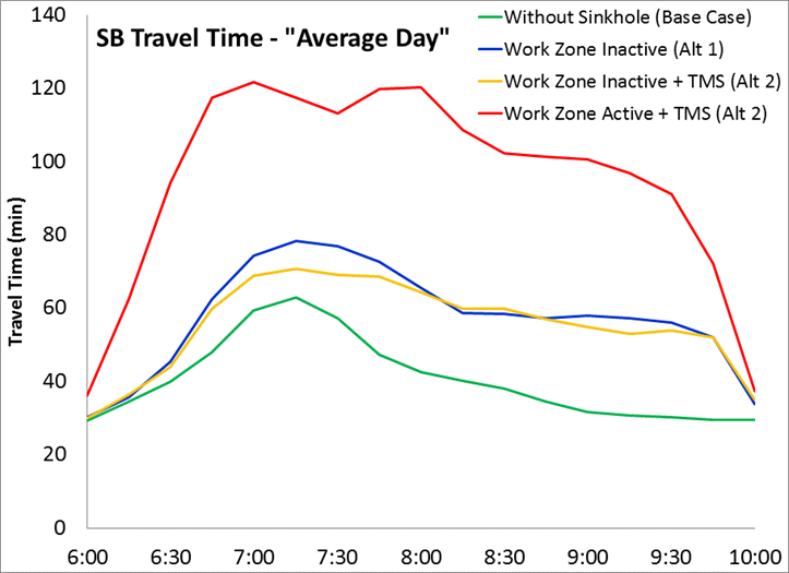
Figure 28. Chart. Travel Time Profiles of Alternatives Total additional delays due to work zones was used as the key performance measure in this alternatives analysis. The total additional delay for Alternative 1 is calculated directly from the work zones inactive condition, i.e., the blue line in Figure 28. The total additional delay for Alternative 2 is calculated from the combination of the two work zone conditions: eighty percent of the delay from work zones inactive with traffic management strategies (yellow line) plus twenty percent of the delay from work zones active with traffic management strategies (red line). The required number of simulation runs for the "average day" case is obtained using the equations provided in Chapter 6. Using four pre-simulation runs yields a result that fewer than four runs are required, therefore four simulation runs will be used. After running simulation four times for both alternatives, Table 18 summarizes the total additional delay calculation during AM peak for the entire work zone period. The Null Hypothesis is set as H0: \(\mu_{1} \leq \mu_{2}\). Using t-test listed in Chapter 6, we do not have enough evidence to reject H0. This implies that when using the traditional "average day" analysis, we cannot statistically determine that Alternative 1 results in lower total additional delay than Alternative 2. Travel Conditions Alternatives Analysis (Follows Updated Guidance) The updated approach gives each travel condition a weight based on how frequently that condition occurs. Therefore, total additional delay is calculated as a weighted sum of delay observed in each travel condition. This allows the analyst to avoid gross generalizations incurred in the "average day" approach when estimating delay. Table 19 presents how delay is calculated in each travel condition. For Alternative 1, the work zone is inactive during the AM peak all the time, while for Alternative 2, the work zone is active under the Low Demand travel condition and the traffic management strategies are applied throughout the entire construction period. Figure 29 and Figure 30 illustrate travel time profiles of different travel conditions. Figure 29 is the SB travel time profile of Low Demand travel condition, where the work zone is inactive in Alternative 1 and active with traffic management strategies in Alternative 2. As expected, activating the work zone on low demand days during AM peak traffic management strategies causes extra delay. Figure 30 is the SB travel time profile of Many Incidents travel condition, where the work zone is inactive in both alternatives and with traffic management strategies applied to Alternative 2. The incident management strategy and demand management strategy in Alternative 2 improve corridor travel time compared to Alternative 1. 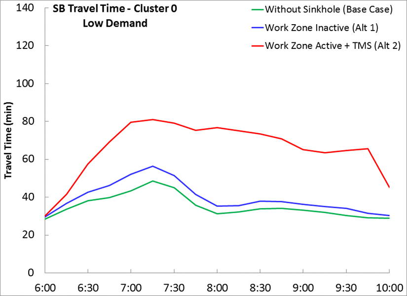
Figure 29. Chart. South Bound Travel Time Profile for Low Demand Travel Condition 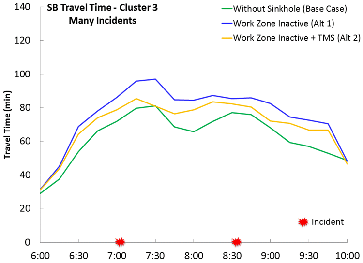
Figure 30. Chart. South Bound Travel Time Profile for Many Incidents Travel Condition Similar to the traditional approach (above), for the travel conditions approach, a calculation should be made to identify the required number of replication. Four simulation runs were found to be sufficient to perform a statistical test in this case. After running the simulation 4 times for each work zone scenario, Table 20 summarizes the total additional delay calculation using the travel conditions approach. In the table, with the additional four work hours logged on low demand days and the time saved to take away and/or setup the work zone, the number of weekdays for Alternative 2 is reduced. The Null Hypothesis is set as H0: \(\mu_{1} \geq \mu_{2}\). Using the t-test listed in Chapter 6, we reject H0. This implies that the total additional delays generated for Alternative 2 is statistically lower than that for Alternative 1. Total Cost Comparison Since Alternative 2 includes the cost of additional traffic management strategies, a further comparison is performed to include both hard and soft costs. Soft cost is the cost due to extra delay; $20/hour is used in this calculation. Hard cost includes both work zone and traffic management strategies costs 1:
Figure 31 depicts the monetized comparison of the two alternatives using different approaches. When considering both hard cost and soft cost with the travel conditions approach, Alternative 2 is still more cost-effective than Alternative 1. 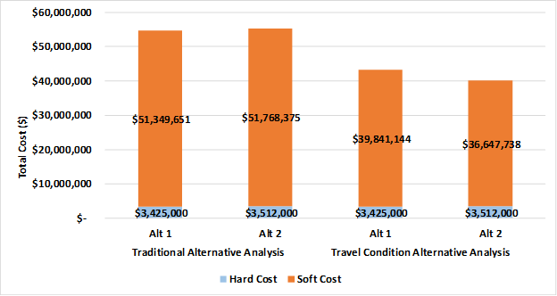
Figure 31. Chart. Total Cost (Hard Cost and Soft Cost) Computation Travel Time Reliability The travel time reliability calculation process is available at the FHWA Office of Operations website: https://ops.fhwa.dot.gov/publications/tt_reliability/. One can calculate travel time reliability with an travel conditions approach. Planning time index is chosen in this case study; that is the 95th percentile travel time divided by the free-flow travel time for each time interval. Figure 32 shows the planning time index plot for NB and SB direction. 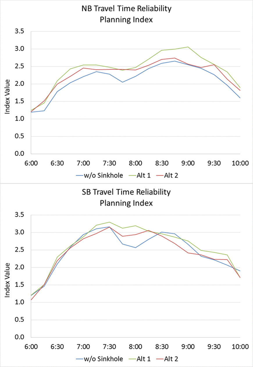
Figure 32. Chart. Planning Time Index In the figures, Alternative 2 has better travel time reliability compared to Alternative 1 in NB direction and Alternative 2 travel time reliability remains at roughly the same level compared to Alternative 1 in SB direction. Therefore, having the work zone active on low demand days does not negatively impact travel time reliability. Conclusion of Alternatives Analysis In summary, Alternative 2 causes more delay in the Low Demand travel condition but this is marginal, and travel time reliability remains at the same level. Alternative 2 also reduces delay under other travel conditions because the traffic management strategies improve overall travel time distributions. When considering both hard and soft costs, using travel conditions approach reveals that the dynamic work zone schedule with supporting traffic management strategies in Alternative 2 is more cost-effective than the fixed work zone schedule in Alternative 1. Furthermore, Alternative 2 shortens the entire construction period by adding more working hours to AM peaks on low-demand workdays. Value of Cluster Analysis A traditional analytical approach focuses on average demand patterns, so the congestion development and dissipation across the full range of observed conditions are not modeled well. That results in unrealistic analyses focused too much on average demand. Cluster analysis provides an approach to focus on time-dynamic data and travel demand in simulation model development and calibration, and thus can provide more accurate assessments to inform decisions. Using cluster analysis to identify travel conditions gives a better representation of system dynamics and underlying causes of congestion and unreliability, while the traditional average day approach only captures "recurrent" conditions that may only rarely occur (less than 30% of days in this case study). In this case study, we demonstrate that without doing the full travel conditions analysis, these case study alternatives cannot be effectively differentiated. This may lead to incorrect information reaching decision-makers. With the full travel conditions analysis, modeling yields a stronger and statistically significant observation to inform decision-makers, i.e., Alternative 2 has lower soft and hard costs, while maintaining system travel time reliability. Overall, considering the results from this case study, the value of the updated guidance on microsimulation may be described as follows:
1 https://ops.fhwa.dot.gov/wz/contracting/index.htm [ Return to Note 1 ] 18 Apache Spark Mllib. https://spark.apache.org/mllib/, Accessed 8 June 2018. [ Return to 18 ] 19 H2O. https://www.h2o.ai/, Accessed 8 June 2018. [ Return to 19 ] 20 TensorFlow. https://www.tensorflow.org/, Accessed 8 June 2018. [ Return to 20 ] 26 PTV VISSIM, http://vision-traffic.ptvgroup.com/en-us/products/ptv-vissim/, Accessed 8 June 2018. [ Return to 20 ] | |||||||||||||
|
United States Department of Transportation - Federal Highway Administration |
||