A Methodology and Case Study: Evaluating the Benefits and Costs of Implementing Automated Traffic Signal Performance
Chapter 2. Relevant Prior Work
This chapter presents background on signal monitoring concepts that enabled automated traffic signal performance measures (ATSPM) to be developed. It also provides an overview of previous studies in which the performance measures were developed and their utility was demonstrated through applications to various real-world use cases.
Event Data Concept
The core data used in ATSPMs is high-resolution data, which is a digital record of events occurring within the signal controller, such as times when signal outputs changed (e.g., transitions between green, yellow, and red for phases or overlaps), detector states changed from "on" to "off" or vice versa, and other control events. In theory, any change in information within a signal controller could be registered as an event. The present enumerations list 101 types of events, and some vendors have independently added more.
In the past, limitations of hardware and communication used in traffic signal systems restricted the availability of detailed data-collection capabilities. Some advanced technologies, such as adaptive signal control, required collection of similar types of data. However, most adaptive systems did not report this internal data. One exception was ACS Lite, whose records of signal and detector state data could be extracted in raw form (Gettman 2007).
In the early 2000s, researchers began to explore use cases in signal control evaluations that required logging of real-time detector and phase states. One use case was the evaluation of new detection systems. The measurement of detector on-time latency made it necessary to record state changes at time resolutions less than 1 second; this led to the creation of an intersection testbed where state changes were logged in real time. Researchers soon realized the data used for evaluating detectors contained useful information for measuring intersection performance (Smaglik 2007; National Transportation Operations Coalition 2012). Around the same time, researchers in Minnesota began to log intersection data in a similar manner, with the goals of evaluating corridor progression by estimating queue lengths to predict travel times of virtual probe vehicles (Liu 2009).
Figure 6 illustrates an example of high-resolution data. In this example, an instance of phase 2 (Φ2) is shown. The time when the controller is managing the timing of phase 2 includes its green, yellow, and red clearance intervals. The start and end of each interval is marked by a corresponding event. The input states of two detector channels are also shown; transitions from an "on" to "off" state, and vice versa, are recorded by events. From these data, assuming the two detector channels represent stop-bar detectors, it's possible to determine when vehicles are waiting for the phase to begin (when the detector turns on), and when the phase is finished serving vehicles (when the detectors turn off).
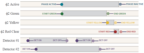 Figure 6. Illustration. Example of states and event data.
Source: FHWA
Figure 6. Illustration. Example of states and event data.
Source: FHWA
Performance Measures and Use Cases
Research into signal performance measures using high-resolution data has been ongoing for more than a decade, and these data have been applied to numerous use cases. A functional classification of use cases for signal performance measures was suggested by researchers (Day 2015), based on the idea that interdependencies of system elements suggest different roles of performance measurement. An illustration of this hierarchy is presented in figure 7; this is slightly modified from earlier representations, reflecting input received from practitioners.
From bottom to top, the five layers are:
- Local control appears at the base of this hierarchy. This represents the phase-switching operation carried out by the local controller, which is the most basic operational function of a traffic signal. As long as the signal has power and appropriate basic programming, it will be able to operate in a rudimentary manner, even if no other part of the system is working. Traffic signal systems are fairly robust in maintaining this basic level of operation.
- Detection is the next layer. Detectors (vehicle and pedestrian) can substantially improve the quality of local control by enabling the controller to adjust green times to match measured traffic demands, thus implementing actuation. Because actuation is only possible if basic local control is also operational, operating detection sits on a higher level in the hierarchy. The quality of local signal operations can be evaluated when the detector information is available.
- Communication comes next; this represents the ability of the local controller to communicate with the outside world. This is needed to synchronize clocks for coordination, and to transmit data externally for performance measurement.
- Coordination is the fourth layer; this represents the operation of multiple intersections in a cooperative manner to promote progressive traffic flows (or other objectives requiring choreography of multiple signal controllers). Coordination depends on the ability of controllers to talk to each other, or at least to receive a common reference time source to remain synchronized. Good quality coordination is also dependent on the functionality of the detection and local control layers.
- Advanced applications is the topmost layer, representing higher-order management applications that could be used in a signalized intersection, such as traffic responsive or adaptive control. The ability of these tools to have a positive impact on system operation is contingent on the working condition of the underlying layers.
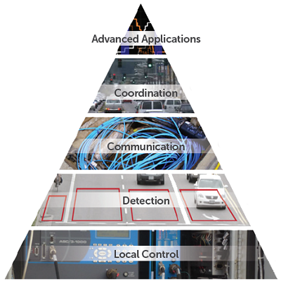
The top layer is entitled “Advanced Applications”, and shows arbitrary statistical charts in the background. The second layer is entitled “Coordination”, and shows vehicles moving through a series of traffic signals in the background. The third layer is entitled “Communication”, and shows blue electrical cables in the background. The fourth layer is entitled “Detection”, and shows rectangular detection zones (near an intersection approach stop line) in the background. The bottom layer is entitled “Local Control”, and shows the inside of a traffic signal controller cabinet in the background.
Figure 7. Illustration. A hierarchical view of signal system functionalities and areas for performance measurement.
Source: FHWA
Each layer has its own maintenance or operation concerns. At a basic level, it is helpful to ensure the system components are functional, such as detection and communication systems. Many agencies invest a lot of time in keeping these systems up and running. The impact of signal timing is also important to quantify; the quality of that service can be described in many different ways, depending on the type of objective of the operation. For example, the distribution of green times affects the service of individual movements; inadequate green time leads to the buildup of vehicle queues; excessive green times on other phases during the same cycles indicate an inefficiency that likely could be corrected.
Table 3 presents a list of objectives for each functional hierarchy layer, with examples of performance measures that have been applied in literature to assist in achieving these objectives. Example studies are highlighted where quantitative user benefits have been demonstrated as an outcome of using performance measures to manage the system. There are only a handful of studies where this is the case; these used external data sources to measure travel times, and converted the change in travel time to annualized user benefits. A few other studies included changes in delay and other similar metrics, but did not include user benefit documentation.
Table 3. Mapping of objectives to performance measures.
| Functional Layer |
Objective |
Performance Measures |
Documented User Benefit |
| Basic Local Control |
Ensure that controllers are functioning. |
Tracking occurrences of intersection flashing operation. |
(Huang 2018) |
| Troubleshoot challenging controller programming. |
Visualization of track clearance operation (Brennan 2010). |
 |
| Timing and actuation diagram (UDOT, n.d.). |
| Detection and Actuated Signal Timing |
Ensure that detectors are not malfunctioning. |
Identification and visualization of failed detectors (UDOT, n.d.; Lavrenz 2017; Li 2013, 2015). |
(Lavrenz 2017) |
| Provide for equitable distribution of green times during undersaturated conditions. |
Volume-to-capacity ratio (Smaglik 2007a; Day 2008, 2009, 2010). |
|
| Green and red occupancy ratios (Freije 2014; Li 2017). |
| Phase termination (Li 2013). |
| Delay estimates from stop-bar detector occupancy (Sunkari 2012; Lavrenz 2015; Smith 2014). |
| Split monitor (UDOT, n.d.). |
| Maximize throughput at the stop bar during oversaturated conditions. |
Throughput (Day 2013). |
|
| Minimize occurrences of red light running. |
Red light running (Lavrenz 2016a). |
| Red and yellow actuations (UDOT, n.d). |
| Provide adequate service to nonmotorized users. |
Conflicting pedestrian volume (Hubbard 2008). |
| Communication |
Ensure that controllers are able to communicate with each other. |
Tracking occurrences of communication loss (Li 2013, 2015; An 2017). |
(Li 2015) |
| Coordination |
Provide timing plans that promote smooth traffic flow. |
Percent on green and arrival type (Smaglik 2007a, 2007b). |
|
| Cyclic flow profile and coordination diagram (Day 2010a, 2011; Hainen 2015; Barkley 2011; Huang 2018). |
(Day 2011) |
| Time space diagram (Zheng 2014, Day 2016). |
|
| Queue length and delay estimates from advance detection (Sharma 2007; Liu 2009; Hu 2013). |
| Estimated travel time (Liu 2009). |
| Decide when to coordinate neighboring intersections. |
Coordinatability index (Day 2011). |
|
| Minimize impacts of excessive queuing during oversaturation. |
Temporal and spatial oversaturation indices (Wu 2010). |
| Advanced Applications |
Assess impacts of adaptive signal control functionalities. |
Various applications of the above metrics (Richardson 2017; Day 2012, 2017). |
|
UDOT = Utah Department of Transportation
The lack of documentation of monetized user benefits does not mean that benefits do not exist. However, for the most part, the extra steps necessary to obtain a quantitative record of such changes is beyond the scope of most studies or agency resources. Directly measuring these changes can be expensive, in that some external method of obtaining travel times is generally needed. It is possible the data itself could provide such estimates, but this has not yet been applied in a conversion to user benefits. Table 4 provides a list of studies that have documented user benefits from studies that provided benefits as an annualized dollar amount.
Table 4. Studies presenting documentation of user benefit from active management of traffic signal systems.
| System Location |
Synopsis |
Amount of User Benefit |
SR 37, Noblesville, IN
(10-intersection corridor) |
Impact of offset optimization for a single time-of-day plan (Day 2011). |
$550,000 ($55,000 per signal) |
| Impact of offset optimization over a 5-year period (Day 2012). |
$3,700,000 ($370,000 per signal) |
| SR 37, Johnson County, IN (11-intersection corridor) |
Repair of broken communication, misaligned time-of-day plan, and offset optimization (Li 2015). |
$3,000,000 ($270,000 per signal) |
| US 421, Indianapolis, IN (X-intersection corridor) |
Repair of broken detection throughout corridor (Lavrenz 2017). |
$900,000 ($150,000 per signal) |
X = number of intersections is unknown.
Implementaton
Activities promoting implementation of traffic signal performance measures were elements of research and development from an early stage. Research in both Indiana and Minnesota led to the development of scalable systems for bringing in field data. In Minnesota, this led to the development of a commercial system, while in Indiana, a prototype system was cooperatively developed between Purdue University and the Illinois Department of Transportation (IDOT). In 2012, Utah Department of Transportation (UDOT) began developing its own system, taking inspiration from the work done in Indiana, and investing considerable resources to develop a stable software package. The code was made available as an open-source license, and offered under the Federal Highway Administration's (FHWA) Open Source Application Development Portal (OSADP) in 2017, when FHWA's fourth Every Day Counts program started. Around this time, UDOT named the overall data and performance measure methodology "automated traffic signal performance measures" (ATSPM).
Indiana's research included outreach to traffic signal vendors. Through collaborative discussions between academia and industry, State, and local agencies, a common data format was agreed upon and became a de facto standard for high-resolution data. By 2016, all major controller manufacturers in the U.S. had implemented high-resolution data collection in at least one model. In addition, third-party vendors had introduced products that could collect high-resolution independent of the controller. Many of these vendors also began to develop their own systems for delivering ATSPMs to the user. At the time of this writing, there are many commercial choices for implementation in addition to the open-source software.
The growth of interest in and development of tools was accelerated in 2014 by the selection of ATSPMs as an American Association of State Highway and Transportation Officials (AASHTO) Innovation Initiative focus technology, and the FHWA's fourth Every Day Counts program in 2017–2018. These programs made hosting numerous workshops possible across the U.S., which increased awareness and implementations of ATSPMs. As of December 2018 (see figure 9), the technology has been implemented by at least 39 State departments of transportation (DOTs) at a demonstration stage, or higher, and institutionalized in four States. Many local agencies have also implemented ATSPMs, or are in the process of doing so. Presently, most of these systems are still in the early phases, many with pilot intersections or corridors with ATSPMs available, but over time the number of intersections has been growing. With ATSPMs themselves having transformed from a research topic to a tool available to practitioners by various means, an emerging focus for new research is utilization of the measures to facilitate performance-based management, as described in Chapter 1: Introduction and Concepts.
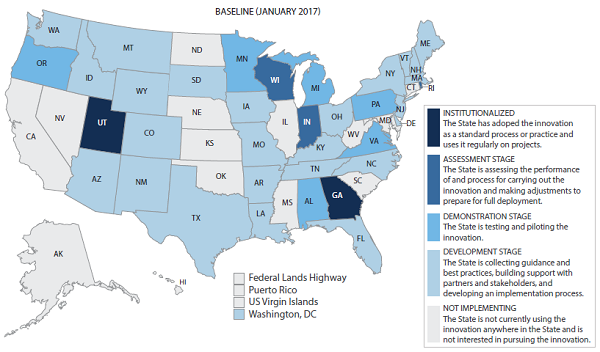
The following five categories of implementation are defined in a color-coded legend: INSTITUTIONALIZED: The State has adopted the innovation as a standard process or practice and uses it regularly on projects. ASSESSMENT STAGE: The State is assessing the performance of and process for carrying out the innovation and making adjustments to prepare for full deployment. DEMONSTRATION STAGE: The State is testing and piloting the innovation. DEVELOPMENT STAGE: The State is collecting guidance and best practices, building support with partners and stakeholders, and developing an implementation process. NOT IMPLEMENTING: The State is not currently using the innovation anywhere in the State and is not interested in pursuing the innovation. The following States are classified as INSTITUTIONALIZED: Utah, Georgia. The following States are classified as ASSESSMENT STAGE: Wisconsin, Indiana, Rhode Island. The following States are classified as DEMONSTRATION STAGE: Oregon, Minnesota, Michigan, Alabama, Virginia, Pennsylvania. The following States are classified as DEVELOPMENT STAGE: Washington DC, Washington State, Idaho, Arizona, Montana, Wyoming, Colorado, New Mexico, Texas, South Dakota, Louisiana, Arkansas, Missouri, Iowa, Kentucky, Tennessee, Florida, North Carolina, Ohio, New York, New Jersey, Delaware, Massachusetts, Vermont, New Hampshire, Maine. The following States are classified as NOT IMPLEMENTING: California, Nevada, Alaska, North Dakota, Nebraska, Kansas, Oklahoma, Illinois, Mississippi, West Virginia, South Carolina, Maryland, Connecticut, Federal Lands Highway, Puerto Rico, US Virgin Islands.
Figure 8. Map. Status of automated traffic signal performance measures implementation in January 2017.
Source: FHWA
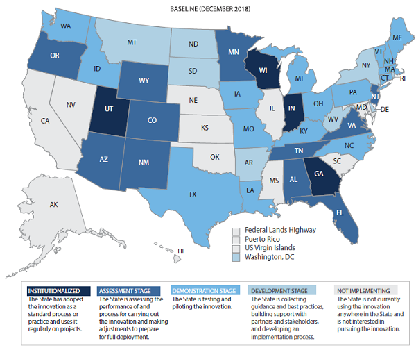
The following five categories of implementation are defined in a color-coded legend: INSTITUTIONALIZED: The State has adopted the innovation as a standard process or practice and uses it regularly on projects. ASSESSMENT STAGE: The State is assessing the performance of and process for carrying out the innovation and making adjustments to prepare for full deployment. DEMONSTRATION STAGE: The State is testing and piloting the innovation. DEVELOPMENT STAGE: The State is collecting guidance and best practices, building support with partners and stakeholders, and developing an implementation process. NOT IMPLEMENTING: The State is not currently using the innovation anywhere in the State and is not interested in pursuing the innovation. The following States are classified as INSTITUTIONALIZED: Utah, Georgia, Wisconsin, Indiana. The following States are classified as ASSESSMENT STAGE: Oregon, Wyoming, Colorado, New Mexico, Arizona, Minnesota, Alabama, Tennessee, Virginia, New Jersey, Florida. The following States are classified as DEMONSTRATION STAGE: Michigan, Pennsylvania, Washington State, Idaho, Texas, Louisiana, Missouri, Iowa, Kentucky, Ohio, North Carolina, Massachusetts, Vermont, New Hampshire, Maine, Connecticut. The following States are classified as DEVELOPMENT STAGE: Rhode Island, Washington DC, Montana, South Dakota, Arkansas, New York, Delaware, North Dakota, West Virginia. The following States are classified as NOT IMPLEMENTING: California, Nevada, Alaska, Nebraska, Kansas, Oklahoma, Illinois, Mississippi, South Carolina, Maryland, Federal Lands Highway, Puerto Rico, US Virgin Islands.
Figure 9. Map. Status of automated traffic signal performance measures implementation adoption in December 2018.
Source: FHWA