A Methodology and Case Study: Evaluating the Benefits and Costs of Implementing Automated Traffic Signal Performance
Chapter 3. Benefit-cost Methodology
Documenting Benefits
According to the theory on diffusion of innovation, transitioning the market share beyond innovators and early adopters involves new technologies to clearly demonstrate quantitative benefits. Similarly, automated traffic signal performance measures (ATSPM) can move beyond qualitative demonstration of benefits (and may clearly demonstrate quantitative benefits) to gain market share among the early majority of the market sector. Many agencies considering adopting ATSPMs want a strong justification before investing resources in the technology. This study proposes a framework for quantifying potential benefits and costs of ATSPMs. There are some challenges in assessing benefits and costs of ATSPMs. At present, there are not enough documented case studies of ATSPM deployments to broadly survey the benefits. This report includes case studies that attempt to improve this body of information; however, few early-adopter agencies have documented their level of quantitative benefits because it is likely unnecessary, given the strong support of executive leadership who understand the enhanced capabilities to improve operations, maintenance, and quality customer service objectives. The amount of quantitative data available is rather limited and in many cases users of the methodology may rely on rough estimates.
Another challenge is that ATSPMs and active management practices represent a fundamental shift in the way systems are operated. Traditional data-collection practices cannot provide the same level of coverage; or, perhaps more accurately, considerably more effort would have to be expended to achieve the same outcome in terms of data collection. Comparisons between traditional practice and active management with ATSPM may consider the increase in an effort required under traditional methods to achieve the same outcome. An analogy can be drawn from pavement management, in which a series of mill-and-overlay activities periodically carried out can maintain higher pavement quality over a longer time period than less-frequent reconstruction. Figure 10 illustrates the difference in outcome over time between proactive and reactive management. The dashed line in the chart shows the background trend in the performance, which in this example shows gradual degradation over time—perhaps this is a corridor where demand is steadily growing. The other lines show the potential performance under proactive or reactive management.
Reactive management reflects the traditional signal retiming practices that produce plans that are narrowly focused, on the peak 15 minutes to 1 hour as an outcome of methods based on a small set of manually collected data. For traffic conditions outside the peak period, the timing is less effective and will result in degraded performance whenever traffic conditions are not consistent with the signal timing optimization design period. This suggests that as traffic demand changes over time, signal timing becomes inappropriate for conditions and will induce degraded intersection performance. In those cases, as the variance in traffic patterns increases, the performance of narrowly focused signal timing plans becomes more recognizable, generally resulting in poor performance and complaints. The effectiveness of the current signal timing practices is thus constrained by limitations in manually collected data and the tools available to process the data.
Proactive management has the potential to sustain performance at a higher level, because issues can be addressed before degradation is prolonged. An agency that proactively manages its signals would not be able to assess its level of performance had they not undertaken that activity. Rather, they may only see the background trend, which as in this example, could reflect a decrease in performance over time. However, the true value of proactive management is avoidance of larger and more rapid decreases that can occur without responsive monitoring.
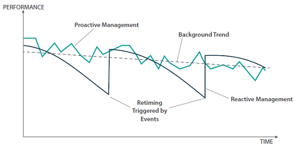
The x-axis is labeled "Time". The y-axis is labeled "Performance". A dashed trendline called "Background Trend" begins at time zero at a fairly high level of performance, and then ends at the maximum time at a slightly lower level of performance. A second trendline called "Reactive Management" also begins at time zero at a fairly high level of performance. Its performance decreases at a more rapid rate until reaching one-third of the maximum time, before shooting straight up to a level slightly lower than the starting level of performance at time zero. Its performance again decreases at a rapid rate until reaching two-thirds of the maximum time, before shooting straight up to a level slightly lower than the level of performance at one-third of the maximum time. Its performance again decreases at a rapid rate until reaching the maximum time. The two instances where performance shot straight up at one-third of the maximum time, and then at two-thirds of the maximum time, are labeled "Retiming Triggered by Events". A third trendline called "Proactive Management" also begins at time zero at a fairly high level of performance. Its performance moves up and down by very small amounts as the trendline extends from left to right, until reaching the maximum time. At all times, the level of performance is never substantially higher or lower than the "Background Trend" trendline.
Figure 10. Graph. Comparison of proactive and reactive management.
Source: FHWA
Variability of timescale of a deployment is another challenge in understanding benefits and costs. Two perspectives can be taken. The first is the potential short-term benefits of improved management in a short time frame after ATSPM deployment. The second is the benefit associated with sustained management of that performance over time. The former can be approached with a traditional before-and-after analysis, while the latter would need to estimate avoided loss in the performance, represented by the area between the reactive management and proactive management curves in figure 10.
Another challenge in assessing benefits and costs of ATSPMs is the overlapping purpose of certain components of the system. It is easy to conflate certain implementation costs (and benefits) with those related to operating a traffic signal system, with or without ATSPMs. The costs of communication and detection—part of the infrastructure of signal systems—are examples. These are both needed for performance measurement, but are also components of the signal system serving purposes that may not have anything to do with performance measurement. Agencies that clearly state operational objectives have a mechanism to drive what infrastructure and technology is required to support attainment of those objectives. This also clarifies the relevant performance measures. While objectives should drive selection of detection and communications needs, it is worthwhile to state that, historically, traffic signals have been treated like commodities and the concept of objectives- and performance-based management is still emerging. As objectives- and performance-based management become normal practices, relevant infrastructure investments (which support both operations and performance monitoring) may become more aligned with objectives and eventually become a standard.
The methodology presented here allows for analysis of benefits and costs from a variety of perspectives, with individual benefit and cost items defined for both short- and long-term time frames. Further, the methodology allows analysts to consider benefits and costs related to ATSPM, but which have a separate operational purpose (such as communication and detection systems). This is intended to permit analysts some flexibility in establishing parameters of their analyses.
Elements of Benefit-cost Analysis
Lists of potential cost (table 5) and benefit items (table 6) are compiled and described in this section. These items were largely identified from documentation in previous studies and one of the authors' previous interactions with agencies that had adopted ATSPMs. Each item is categorized according to its scope: short-term, long-term, or both. The benefit and cost items are further sorted into categories and benefit-cost types.
Cost types refer to the type of investment incurring the cost, such as:
- Labor—direct use of personnel time by the agency.
- Equipment—procurement and installation of new devices, parts, software, etc., for effective utilization of the ATSPM.
- Infrastructure—procurement of traffic signal control equipment. In many cases existing equipment may be used; new equipment procured may deliver its own benefits to the operation independent of ATSPM use. This scenario is discussed later in the paper.
Benefit types include benefits to the public and agency. Public benefits are further categorized among the potential ways they can materialize, such as:
- Travel time (TT)—the public incurs less delay when traveling on signalized facilities.
- Crash reduction (CR)—risk of crashes is reduced.
Table 5. List of cost items.
| Line |
Scope |
Category |
Item |
Cost Type |
| 1 |
S |
Data logger |
Procuring new controllers or controller add-on equipment/firmware. |
Labor, infrastructure |
| 2 |
S |
Data logger |
Updating existing controller firmware. |
Labor |
| 3 |
S |
Data logger |
Procuring external data collection devices. |
Labor, infrastructure |
| 4 |
S |
Communication |
New communication system added. |
Infrastructure |
| 5 |
L |
Communication |
Communication system maintenance. |
Infrastructure |
| 6 |
S |
Detection |
New detection systems added. |
Infrastructure |
| 7 |
L |
Detection |
New detection systems added. |
Infrastructure |
| 8 |
S |
Detection |
Reconfiguration of existing detection systems. |
Labor, equipment |
| 9 |
S |
Detection |
Documentation of detector assignments. |
Labor |
| 10 |
S |
Server |
New server procurement. |
Equipment, labor |
| 11 |
S |
Server |
Server maintenance and database management. |
Labor |
| 12 |
S |
Software |
Software license cost. |
Equipment |
| 13 |
S |
Software |
Installation cost. |
Labor |
| 14 |
L |
Software |
Maintenance and troubleshooting. |
Labor |
| 15 |
S |
Integration |
Business process integration. |
Labor |
| 16 |
L |
Integration |
Active ATSPM management/operations cost. |
Labor |
ATSPM = automated traffic signal performance measures. S = short term. L = long term.
Table 6. List of benefit items.
| Line |
Scope |
Category |
Item |
Benefit Type |
| 1 |
L |
Organizational |
Avoidance of manual data collection. |
Agency |
| 2 |
L |
Organizational |
Avoidance of unneeded retiming/maintenance activities. |
Agency |
| 3 |
L |
Organizational |
Reduced public complaint response time. |
Agency |
| 4 |
L |
Organizational |
Value of performance documentation. |
Agency |
| 5 |
Both |
Maintenance |
Discovery and repair of failed detectors. |
Public (TT) |
| 6 |
Both |
Maintenance |
Discovery and repair of broken communication. |
Public (TT) |
| 7 |
Both |
Maintenance |
Discovery and repair of other equipment failures. |
Public (TT) |
| 8 |
Both |
Operations |
Discovery and resolution of inefficient green distribution. |
Public (TT) |
| 9 |
Both |
Operations |
Discovery and improvement of poor coordination. |
Public (TT) |
| 10 |
Both |
Operations |
Discovery and mitigation of pedestrian operational issues. |
Public (TT) |
| 11 |
Both |
Operations |
Discovery and resolution of preemption-related issues. |
Public (TT) |
| 12 |
Both |
Operations |
Identification of locations with potential safety issues. |
Public (CR) |
CR = crash reduction. L = long term. TT = travel time or delay.
It should be noted that not every cost and benefit may occur in any given ATSPM deployment. In particular, the benefits could align with agency objectives as appropriate to an agency's signal management plan or other strategic planning documents. For example, an agency whose objectives primarily focus on improving signal timing practices regarding its pedestrian operation may not wish to include a coordination-related improvement, particularly if those aspects of operation will not be analyzed by performance measures, or are otherwise unlikely to drive action.
The following sections present notes on each item in turn. First, agency cost items are discussed, followed by benefit items. Where previous studies have quantified the amount of benefit on a specific item, notes from the relevant documentation are included.
Potential Costs of Automated Traffic Signal Performance Measures
Procuring new controllers or controller add-on equipment/firmware. Where existing equipment does not provide the ability to log high-resolution data, new controllers may be acquired, or, in some cases, existing controllers can be upgraded with new add-on equipment (such as a physical module) or firmware that may incur cost. These will incur a certain unit cost, typically between $2,500 and $5,000 at the time of writing, but often influenced by quantity of units procured. Newer traffic signal controllers may bring other added functionality beyond the ability to collect high-resolution data, so they are considered an infrastructure cost type.
Updating existing controllers. Many existing traffic signal controllers can log high-resolution data. Sometimes a firmware upgrade and additional configuration steps are needed to turn on the controller logging capability. These activities require personnel time investment to accomplish; there may be an additional cost, depending on the specific relationship of the agency to its vendors and distributors.
Procuring external data-collection devices. As an alternative to controller-based data loggers, several different commercial devices have been developed by vendors to collect high-resolution data. Some devices may provide additional functionality beyond data collection, and, therefore, are included in the infrastructure category. The addition of probe vehicle data (and other external data sources) might also be considered; cost for that data would fall under this category.
New communication system added. Some form of communication infrastructure is typically needed for coordinated traffic signal systems. Communication systems are also needed to automatically harvest high-resolution data for ATSPMs; in particular, these must permit transmission of the data. Therefore, in some cases an upgrade may be needed to allow for ATSPMs to be deployed. This is considered an infrastructure cost. Where no communications to a central system is available, an alternative approach would be to manually retrieve the data at intervals (e.g., once a week, month, etc.). Such costs should be included here.
Communication system maintenance. As noted above, communication systems are necessary for both traffic signal control and ATSPM deployment. Maintenance of such systems is necessary and also listed as an infrastructure cost.
New detection systems added. Similar to communication systems, detection systems have a primary use in traffic signal control, but may also be used for data-collection purposes. Certain types of ATSPM analyses are only possible with certain types of detection. For example, to measure vehicle arrivals, advance detection is needed (other types of analysis are still possible without it). Detection may sometimes be added in conjunction with an ATSPM deployment. However, since new detection can potentially be used to improve traffic signal operation independent of ATSPMs, it is listed here as an infrastructure cost.
Detection system maintenance. Similar to communication systems, new detection systems will bring maintenance needs. This is listed as an infrastructure cost as well; such items may be conflated with the cost needed primarily for ATSPMs. This is discussed in detail later in the primer.
Reconfiguration of existing detection systems. The configuration of existing detection zones has an influence on the outcomes of an ATSPM analysis. In some cases, the agency may wish to reconfigure its detection zones to improve the quality of performance measures. For example, some agencies may combine many detection zones on a single channel to simplify how detection zones are received by the controller (e.g., channels 1–8 mapped to phases 1–8). This can cause problems with data analysis. For example, a channel that combines both advance and stop-bar detectors cannot provide accurate arrival information. In such cases it may be possible to reconfigure the detection zones to separate channels. Regardless of whether such reconfiguration is needed, documentation of detector channel assignments is also desired for most performance measures. Sometimes this may involve only labor cost (e.g., changing video detection zones). In other cases, some equipment cost may be used (e.g., resplicing loops).
Documentation of existing detection systems. Most ATSPMs (one exception being a phase termination analysis) involve documenting and entering the detector mapping into the performance measurement system. Agencies vary considerably in their practices of documenting detector configurations. In some cases, agencies may already possess a database that stores each intersection's configuration in detail. In other cases, the information may not be readily available. Some amount of labor may be needed to capture the detector assignments for purposes of developing ATSPMs. In general, many agencies have found this cost to be quite unexpected because many States' design documents delegate detector number and configuration to signal technicians and drawings, which only reside in the cabinet as sketches.
New server procurement. A system for data storage, processing, and delivery of ATSPMs may be used. In some cases, new server hardware may be used. In other cases, existing server hardware could be leveraged. Another option is to use cloud computing rather than conventional server hardware. In any case, some cost may be applied toward procurement. Some labor cost may also be applied toward server installation and configuration.
Server maintenance and database management. In addition to procurement costs, a server may bring related maintenance costs; service fees would likely apply for cloud computing. This line item reflects such costs.
License costs for existing systems. Some commercial ATSPM systems (or add-on modules to ATMS or other existing systems) may require a license cost. These may be subscription-based or one-time costs, or follow a different pricing model. These costs would not be incurred with opensource software (although that could incur higher installation costs).
Installation cost. This item reflects the labor needed to install the software for an ATSPM system. For commercial systems this likely will be lower than open-source software.
Maintenance and troubleshooting. This pertains to labor costs specifically needed to maintain the ATSPM software over time. This may be rolled up into the procurement cost for commercial systems. Users of open-source software may incur a cost associated with upgrading to newer versions over time.
Business process integration. Agencies may consider how ATSPMs will fit in their overall programs, and plan for some costs related to integrating them into day-to-day activities, such as training programs or integration into existing agency procedures and manuals. The Federal Highway Administration's (FHWA) Traffic Signal Capability Maturity Framework (FHWA 2016) provides the following model for describing levels of integration:
- Level 1, ad hoc (low capability).
- Level 2, managed (medium capability).
- Level 3, integrated (high capability).
- Level 4, optimized (highest capability).
An ATSPM deployment championed by a few individuals in an agency is unlikely to advance beyond level 1, and that capability may evaporate if those individuals leave the agency or move to other positions. Some costs associated with effort to achieve at least the third level of capability may be considered.
Active ATSPM management/operations cost. This is the cost of staff who monitor and fix signal timings in the ATSPM software when such activities are not invoked by external complaints. The amount of time spent using ATSPM may be balanced against time invested in other activities to accomplish the same purpose. This cost category is a counterpart of the traditional method of retiming traffic signals on arbitrary schedules (e.g., once every few years), which is reflected in the benefit category of "avoidance of unneeded retiming/maintenance activities" described in the next section.
Potential Benefits of Automated Traffic Signal Performance Measures
Avoidance of manual data collection. Traditionally, many agencies have relied on manual data collection to develop turning movement counts at intersections. In current practice it is becoming common to use automated systems to develop such data, with counting devices temporarily deployed. Another common traffic study method is to use tube counters to develop average daily traffic (ADT) for links. ATSPMs can facilitate use of detectors to provide count data, potentially reducing the need for other count methods. Floating-car studies or other methods of travel time data collection might be eliminated with data sets such as probe vehicle data.
Avoidance of unneeded retiming/maintenance activities. Without performance monitoring, agencies often rely on scheduled maintenance and retiming activities to manage their systems. This means these activities are performed whether or not they are needed. By shifting to performance-based monitoring, some of these activities can be reduced.
Reduced public complaint response time. Many agencies spend considerable effort responding to public calls about traffic signal operation. Common examples include excessive delay spent at a location, or apparently malfunctioning signals. These calls can require a lot of time to track and troubleshoot, particularly with intermittent problems or those that occur outside ordinary working hours. ATSPMs can simplify these identification tasks. They can also be used to verify that a problem has been addressed. In addition, ATSPMs may also be able to help an agency proactively identify and mitigate situations that generate complaint calls.
Value of performance documentation. ATSPMs introduce some capability to document system performance, including both current performance and how that trends over time. This may provide opportunities to improve public relations of the agency and to document needs or show return on investment to decision makers. An example is the Utah Department of Transportation (UDOT) statistic in the following headline: "Odds of hitting a red light in Utah? Just 1-in-4" (Davidson 2013).
Discovery and repair of failed detectors. ATSPMs can improve management of vehicle detectors, pedestrian buttons, and similar actuation devices. Failed detectors can have a substantial impact on traffic signal operation, since they often must be compensated with default to fixed-time operation on the affected movements. A comprehensive evaluation of the cost of failed detection has not been done, but "wasting" green time on movements that may not have demand can increase delays on all other movements at the affected intersection. A study in Indiana (Day et al., 2015) found that for a single corridor, annualized benefits of $900,000 were realized through detector repairs. In that study, seven different detectors had failed at the six-intersection corridor.
Discovery and repair of broken communication. Maintaining working communication is helpful to keeping controller clocks synchronized, which is helpful for coordination. ATSPM systems can facilitate better management of communication links to intersections. A study by Li et al. (2015) assessed user benefits from the repair of communication failures, finding an annualized user benefit of about $420,000 for a corridor with 12 intersections. This benefit was assessed by examining the difference in median travel times before and after correction of issues that led to incompatible patterns being run at neighboring intersections.
Discovery and resolution of inefficient green distribution. Allocation of capacity by the distribution of green times is a key operational function of traffic signals; inefficiencies in green time distribution can accumulate delay. ATSPMs include metrics that can be used to assess whether individual movements are experiencing degraded performance and if green times can be reallocated to address these issues, potentially reducing delays. Freije et al. (2014), for example, examined a chance in the number of split failures before and after the implementation of a split change. That study did not directly examine the conversion of such numbers to a numerical benefit; Smith (2014) explored a delay estimate. The next section describes potential ways to estimate such benefits in greater detail.
Discovery and improvement of poor coordination. Another key aspect of traffic signal operation is the achievement of progression with coordination. Poor quality progression may occur due to the provision of offsets that are poorly suited to the traffic conditions. This may occur for a variety of reasons, such as divergence in traffic patterns over time; an example would be a change in how often a side-street phase gaps out—which leads to a change in early return to green and consequently the arrival and departure patterns of vehicles. A study by Lavrenz et al. (2015a) examined the management of traffic signal offsets over a 5-year (yr) period through use of ATSPMs and three separate retiming activities on a corridor experiencing a 36 percent increase in volumes during that time period. When the changes in travel time and travel time reliability were converted into annualized user benefits, a total of about $3.7 million was estimated over the 5-yr period. This was a corridor of nine intersections. The previously mentioned study by Li et al. (2015) attributed $2.9 million in annualized benefits to an improvement of offsets on a 12-intersection corridor.
Discovery and mitigation of pedestrian operational issues. Locations with high pedestrian delay can be identified using ATSPMs; one way to identify this is examining the time to service for pedestrian calls. This may lead to potential improvements in traffic signal timing; to date, this use case has not been explored in detail.
Discovery and resolution of preemption-related issues. Preemption and priority control at traffic signals can sometimes require complex configuration, and includes interfacing with equipment of other entities or organizations (railroad operators, emergency services, transit operators, etc.). The ability to identify and mitigate issues is a potential use case of ATSPM. An example presented by UDOT demonstrated the use of ATSPM to evaluate a public complaint about malfunctioning railroad preemption. Performance measures were able to reveal that an excessive number of preemptions were occurring, which was rectified by making the railroad operator aware of the issue.
Identification of locations with potential safety issues. One potential benefit of ATSPMs is their application to intersection safety. At present, this potential use has not been extensively explored. The UDOT open-source software allows detector actuations during red to be visualized, which can serve as a screening tool for identifying locations for enforcement. Lavrenz et al. (2015b) developed an estimate of the number of red light violations, and examined how the estimate changed after a split adjustment was made. Hubbard et al. (2008) investigated a measure of vehicle-pedestrian conflict by considering the amount of conflicting vehicular flow coincident with pedestrian calls for service, which seems likely to correlate with pedestrian-vehicle conflicts. In practice, identifying high-risk locations might lead to countermeasures that may reduce the number of crashes. Some countermeasures may involve further investments (e.g., changing intersection configuration), but there is some value associated with discovery of those issues. Crash reductions related to changes in traffic signal timing would be more appropriate to attribute to ATSPM.
Assessing Benefits and Costs of Infrastructure Investments beyond Automated Traffic Signal Performance Measures
Some cost items in the preceding analysis were identified as improvements in traffic signal infrastructure. While some of these costs are needed to allow ATSPM deployment, the improvements also have intrinsic value independent of ATSPM deployment. For example, installing a detection system at an intersection that does not have one would enable actuation, and, therefore, allow the operation to be changed from fixed-time to actuated control. This operational change would see some differences in the system performance independent of ATSPM.
The degree to which this issue will affect a benefit-cost analysis will largely depend on the starting point of the agency seeking to deploy ATSPM. Agencies that have previously invested in detection systems to obtain coverage of most movements, or communication systems that can reach most intersections, will not have to make many investments of this type. Other agencies that have not had such practices may need to make this investment. For example, the Indiana Department of Transportation (INDOT), one of the earliest users of ATSPMs, had existing standard detector design practices that allowed for stop-bar detection on all minor phases at every intersection, with advance detection on all major phases. In this case, all that was needed to implement ATSPMs was a controller that could collect data and a means of retrieving the data. Not all agencies that have adopted ATSPMs are working from a similar starting point.
The present methodology assumes that it may be possible to attribute portions of the cost to ATSPMs. It is challenging to develop guidance on how such portions should be attributed, and it will likely have to be considered on a case-by-case basis. For example, the case of installing new detection will incur some cost; the agency may choose to consider that cost fully as part of ATSPMs, a separate cost item, or some percentage split between the two. Another option is that such costs would have been encountered as part of upgrading or maintaining the traffic signal system independent of the ATSPM effort; these could be considered sunk costs that can be excluded from the benefit-cost analysis since they were already spent, or would have been expended even if ATSPMs were not implemented. Ultimately the decision to include these cost items must be made by the analyst in computing benefits and costs. A key consideration in how costs are attributed is the purpose and need associated with funding that is acquired to support implementation. If the purpose and need of the funding are expressly identified to implement ATSPM, then devices and infrastructure procured and installed that enhance operations could be attributed to ATSPM implementation. If the purpose and need of funding acquired are expressly identified to provide for intersection operational improvements, then associated cost for devices and infrastructure need not be attributed as cost for ATSPM, and instead may be considered as sunk cost. If purpose and need for funding support both operational improvements and ATSPM, then the cost could be divided and attributed appropriately. These choices are at the discretion of the evaluator. The following methodology seeks to estimate benefits of ATSPM deployments without regard to unrelated benefits of adding new technology such as detection. This part of the analysis assumes that the intersections have already been brought to the point where ATSPMs can be implemented, although in practice that may not be the case. When measuring changes in performance under these circumstances, the analyst may bear this in mind.
Methodology
The benefit-cost methodology consists of two major steps. The first step is to quantify the amount of cost or benefit for each item identified in the first section. For this report, these items have been defined with the assumption that it will be possible to yield realistic estimates of their value. At the time of writing, there are few existing studies where such estimates have been explored, so this is an area where further research is desired. The second step is to total the benefits and costs to estimate the net value.
This methodology intends to produce a benefit-cost analysis over a design life. The user may define that design life; the examples presented here consider a life of 10 years. Depending on whether that value is too long or too short, it can be adjusted. The analysis could also be shortened to only consider short-term benefits, as a more limited before-and-after study, by excluding long-term elements. It should be noted the long-term benefits, in particular, are not well-documented by previous studies, and their analysis will have to heavily rely on broad estimates.
Some benefit and cost items are envisioned as short-term benefits mostly incurred at the beginning of implementation. Many one-time costs to procure and install system components fall in this category. Similarly, an increase in user benefits often can be anticipated shortly after implementation due to discovery of maintenance problems and operational inefficiencies that were unknown before data about the system could be obtained. The long-term benefits and costs are due to recurring maintenance costs per year and recurring benefits from changes in practice.
Cost Items
The total estimated cost is the sum of the line items in table 5:
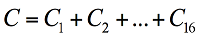
Equation 1
C1 is the procurement cost of controller improvements or upgrades:
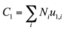
where Ni is the number of intersections of controller type i, and ul,i is the cost associated with readying a controller of type i for ATSPM. Where the controller must be replaced, that cost would be equal to the cost of replacement with a new controller.
Equation 2
C2 is the labor cost of upgrading controller firmware:
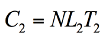
where N is the number of intersections affected, L2 is the labor cost per hour, and T2 is the number of person-hours per intersection.
Equation 3
C3 is the procurement cost of external data logging devices:
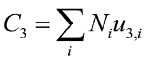
where Ni is the number of intersections to be equipped with device of type i, and u3,i is the unit cost of device type i.
Equation 4
C4 is the cost of communication system development:
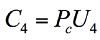
where Pc is the percentage of communication infrastructure cost attributable to ATSPM and U4 is the unit cost of the infrastructure investment.
Equation 5
C5 is the cost of communication system maintenance:
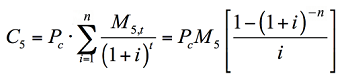
The term is a quotient. The numerator of the quotient is (M subscript 5,t). The denominator of the quotient is the quantity (1 plus i) raised to the power of t. The cost of communication system maintenance (C subscript 5) is also equal to the product of (P subscript c), (M subscript 5), and a third term. The third term is a quotient. The numerator of the quotient is 1 minus the quantity (1 plus i) raised to the power of negative n. The denominator of the quotient is i.
where Pc is the percentage of communication infrastructure cost attributable to ATSPM; M5,t is the value of maintenance costs during year t, summed over years 1 through n, using interest rate i for determining net present value; and M5 is used if the same cost is assumed for each year.
Equation 6
C6 and C7 can be defined similarly:

Equation 7
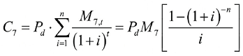
The cost of detection system maintenance (C subscript 7) is equal to the product of (P subscript d) and summation of terms across all values of i from 1 to n. The term is a quotient. The numerator of the quotient is (M subscript 7,t). The denominator of the quotient is the quantity (1 plus i) raised to the power of t. The cost of detection system maintenance (C subscript 7) is also equal to the product of (P subscript d), (M subscript 7), and a third term. The third term is a quotient. The numerator of the quotient is 1 minus the quantity (1 plus i) raised to the power of negative n. The denominator of the quotient is i.
where Pd is the percentage of detection infrastructure cost attributable to ATSPM; M6 is the total cost of new detection; M7,t is the value of maintenance costs during year t, summed over years 1 through N, using interest rate i; and M7 can be used if the same cost is assumed for each year.
Equation 8
C8 is the cost of detection system reconfiguration:
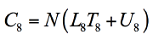
where N is the number of intersections affected, L8 is the labor cost per hour, and T8 is the number of person-hours per intersection needed. U8 is the total equipment cost (if any) required to accomplish reconfiguration.
Equation 9
C9 is the labor cost of documenting the detection configurations:

where N is the number of intersections affected, L9 is the labor cost per hour, and T9 is the number of person-hours per intersection needed.
Equation 10
C10 is the cost of a new server procurement. This is a single-unit cost specific to the site. In some cases, the agency may be able to leverage an existing server and would not incur a cost.
C11 is the cost of server maintenance over the analysis period:
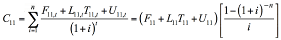
The cost of server maintenance over the analysis period (C subscript 11) is equal to the summation of a quotient across all values of i from 1 to n. The numerator of the quotient is (F subscript 11,t) plus (U subscript 11,t) plus the product of (L subscript 11,t) and (T subscript 11,t). The denominator of the quotient is the quantity (1 plus i) raised to the power of t. The cost of server maintenance over the analysis period (C subscript 11) is also equal to the product of two terms. The first term is the quantity of (F subscript 11) plus (U subscript 11) plus the product of (L subscript 11) and (T subscript 11). The second term is a quotient. The numerator of the quotient is 1 minus the quantity (1 plus i) raised to the power of negative n. The denominator of the quotient is i.
where F11,t is the value of the annual fee, L11,t is the labor cost per hour, T11,t is the total number of person-hours, and U11,t is the unit cost of hardware replacements, for year t, summed over years 1 through n, with interest rate i. The terms F11, L11, T11, and U11 can be used if these quantities are assumed to be the same during each year.
Equation 11
C12 is the cost of a software license:
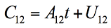
where A12 is a subscription-based cost of a system (if any), t is the number of time units associated with it (i.e., number of payments made, most likely annually), and U12 is a one-time unit cost (if any) of the license.
Equation 12
C13 is the installation cost of the software. The cost to the agency could be 0, for example, if it is rolled into a system procurement. In cases where labor is required, it could be estimated from the following expression:
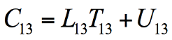
where L13 is the labor cost per hour, T13 is the number of person-hours required, and U13 is a one-time unit cost (if any) of software installation.
Equation 13
C14 is the cost of maintaining the software. There may be no such cost to the agency if the cost is included in a system procurement. The following expression considers the possibility of a recurring cost for maintenance:
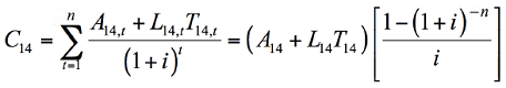
The cost of maintaining the software (C subscript 14) is equal to the summation of a quotient across all values of t from 1 to n. The numerator of the quotient is (A subscript 14,t) plus the product of (L subscript 14,t) and (T subscript 14,t). The denominator of the quotient is the quantity (1 plus i) raised to the power of t. The cost of maintaining the software (C subscript 14) is also equal to the product of two terms. The first term is the quantity of (A subscript 14) plus the product of (L subscript 14) and (T subscript 14). The second term is a quotient. The numerator of the quotient is 1 minus the quantity (1 plus i) raised to the power of negative n. The denominator of the quotient is i.
where A14,t is an annual subscription-based cost for system maintenance (if any), L14,t is the labor cost per hour, and T14,t is the number of person-hours required, for year t, summed over years 1 through n, with interest rate i. The terms A14, L14, and T14 can be used if these quantities are assumed to be the same during each year.
Equation 14
C15 is the cost associated with business process integration. C16 provides an estimate of the amount of effort associated with use of ATSPMs in the long term to achieve the benefits. These are considered as labor costs, formulated similarly to other such costs:
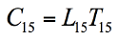
Equation 15
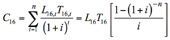
The estimated long-term management and operations cost to achieve the benefits of automated traffic signal performance measures (C subscript 16) is equal to the summation of a quotient across all values of t from 1 to n. The numerator of the quotient is the product of (L subscript 16,t) and (T subscript 16,t). The denominator of the quotient is the quantity (1 plus i) raised to the power of t. The estimated long-term management and operations cost to achieve the benefits of automated traffic signal performance measures (C subscript 16) is also equal to the product of two terms. The first term is the product of (L subscript 16) and (T subscript 16). The second term is a quotient. The numerator of the quotient is 1 minus the quantity (1 plus i) raised to the power of negative n. The denominator of the quotient is i.
where L15, L16,t are the labor cost per hour, and T15, T16,t is the number of person-hours required. In the case of C16, the annual costs are established for year t = 1 through n, with interest rate i. The terms L16 and T16 can be used if these quantities are assumed to be the same during each year.
Equation 16
Benefit Items
The total estimated benefit is the sum of line items in table 6:
Equation 17
The first four benefit items are long-term items; for each of these, the equations are set up to find the net present value for years 1 through n, at interest rate i.
B1 is the benefit associated with the reduction of agency labor used for manual data collection:
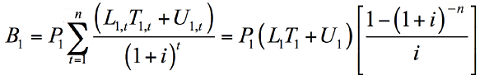
The benefit associated with the reduction of agency labor used for manual data collection (B subscript 1) is equal to the product of (P subscript 1) and summation of terms across all values of t from 1 to n. The term is a quotient. The numerator of the quotient is (U subscript 1,t) plus the product of (L subscript 1,t) and (T subscript 1,t). The denominator of the quotient is the quantity (1 plus i) raised to the power of t. The benefit associated with the reduction of agency labor used for manual data collection (B subscript 1) is also equal to the product of three terms. The first term is (P subscript 1). The second term is the quantity of (U subscript 1) plus the product of (L subscript 1) and (T subscript 1). The third term is a quotient. The numerator of the quotient is 1 minus the quantity (1 plus i) raised to the power of negative n. The denominator of the quotient is i.
where P1 is the overall percentage reduction in manual data-collection activities, L1,t is the unit cost of labor associated with these activities, and T1,t is the total number of person-hours dedicated to these activities. U1,t represents cost reduction from data-collection equipment that may not be needed if ATSPM replaces it. These occur in year t, with interest rate i. The terms L1, T1, and U1 can be used if these quantities are assumed to be the same during each year.
Equation 18
B2 and B3 are the labor savings from a reduction in person-hours needed for the respective tasks of arbitrarily scheduled maintenance or retiming, or responding to complaint calls. These are formulated similarly:
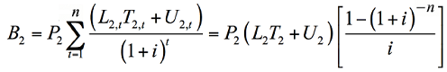
The benefit associated with labor savings from a reduction in person-hours needed for arbitrarily scheduled maintenance or retiming (B subscript 2) is equal to the product of (P subscript 2) and summation of terms across all values of t from 1 to n. The term is a quotient. The numerator of the quotient is (U subscript 2,t) plus the product of (L subscript 2,t) and (T subscript 2,t). The denominator of the quotient is the quantity (1 plus i) raised to the power of t. The benefit associated with labor savings from a reduction in person-hours needed for arbitrarily scheduled maintenance or retiming (B subscript 2) is also equal to the product of three terms. The first term is (P subscript 2). The second term is the quantity of (U subscript 2) plus the product of (L subscript 2) and (T subscript 2). The third term is a quotient. The numerator of the quotient is 1 minus the quantity (1 plus i) raised to the power of negative n. The denominator of the quotient is i.
Equation 19
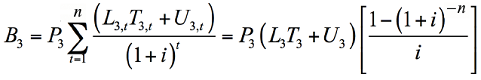
The benefit associated with labor savings from a reduction in person-hours needed for responding to complaint calls (B subscript 3) is equal to the product of (P subscript 3) and summation of terms across all values of t from 1 to n. The term is a quotient. The numerator of the quotient is (U subscript 3,t) plus the product of (L subscript 3,t) and (T subscript 3,t). The denominator of the quotient is the quantity (1 plus i) raised to the power of t. The benefit associated with labor savings from a reduction in person-hours needed for responding to complaint calls (B subscript 3) is also equal to the product of three terms. The first term is (P subscript 3). The second term is the quantity of (U subscript 3) plus the product of (L subscript 3) and (T subscript 3). The third term is a quotient. The numerator of the quotient is 1 minus the quantity (1 plus i) raised to the power of negative n. The denominator of the quotient is i.
where P2, P3 are the overall percentage reduction in the associated task, L2,t, L3,t are the unit cost of labor appropriate to each task, and T2,t, T3,t are the total number of person-hours dedicated to each task. Terms U2,t, U3,t reflect the potential costs for agencies that contract these activities to consultants and for which the cost may be better estimated as a unit cost totaled over the time period, as opposed to a labor cost. As before, these each occur in year t, while the terms L2, L3, T2, T3, U2, and U3 can be used if these quantities are assumed to be the same during each year.
Equation 20
B4 is the value of performance documentation. It does not necessarily represent a labor reduction. This is a difficult cost to express monetarily; the value would strongly depend on the specific needs of the agency performing the analysis. An example of a quantitative benefit related to this would be the ability of the agency to successfully request funds with the help from data documented by ATSPMs. If considered as a recurring annual benefit, it could be converted into net present value as shown earlier.
B5 through B11 are the public benefits that have both a short- and a long-term component, as well as a reduction in complaint calls and travel times or delays. The following equation is proposed to encapsulate all three aspects. It is intended to be calculated for different roadway elements—either routes or movements, as appropriate:
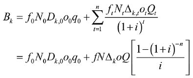
The public benefits having both a short- and a long-term component, as well as a reduction in complaint calls and travel times or delays, is denoted as (B subscript k). (B subscript k) is equal to the summation of two quantities. The first quantity is the product of (f subscript 0), (N subscript 0), (D subscript k,0), (o subscript 0), and (q subscript 0). The second quantity is a summation of terms across all values of t from 1 to n. The term is a quotient. The numerator of the quotient is the product of (f subscript t), (N subscript t), (? subscript k,t), (o subscript t), and (Q subscript t). The denominator of the quotient is the quantity (1 plus i) raised to the power of t. (B subscript k) is also equal to the summation of two quantities. The first quantity is the product of (f subscript 0), (N subscript 0), (D subscript k,0), (o subscript 0), and (q subscript 0). The second quantity is the product of two terms. The first term is the product of f, N, (? subscript k), o, and Q. The second term is a quotient. The numerator of the quotient is 1 minus the quantity (1 plus i) raised to the power of negative n. The denominator of the quotient is i.
In the above, k = 5, 6, … 11 indicates a specific benefit item as described in table 6.
The first term is the short-term component:
- f0 is the value associated with a unit of delay in year 0.
- N0 is the number of elements affected in year 0.
- Dk,0 is the average delay reduction per roadway element associated with short-term gains shortly after deployment.
- o0 is the average vehicle occupancy for year 0.
- q0 is the average flow rate per movement in year 0.
The second term is the long-term component:
- ft is the value associated with a unit of delay in year t.
- Nt is the number of coordinated routes affected during year t.
- Δk,t is the total avoided performance loss per route during year t.
- ot is the average vehicle occupancy for year t.
- Qt is the average flow rate per route associated with long-term avoidance of performance loss during year t.
Equation 21
As before, if the above five quantities are assumed to be the same for each year in the analysis period, then the form of the equation using f, N, Δ, o, and Q can be used.
It is intended the above would be applied either for individual movements or individual routes, depending on whether the benefit is accumulated for individual movements or along routes. Benefits B6 and B9 are probably best considered on the basis of routes; the others would be better estimated in terms of movements.
The above estimate could be tabulated on a per facility basis, e.g., summing for each movement and route at locations where ATSPMs are to be deployed. For estimates considering a broad deployment affecting many movements and routes, it may be more expedient to come up with nominal values for typical movements and routes.
One other detail is that of vehicle classes. For different vehicle classes, different values of f and o would be applicable. That is, a separate analysis could be done for passenger cars, buses, trucks, etc., according to the breakdown of users on the roadway.
B12 is the value of safety improvements facilitated through ATSPM. As mentioned earlier, this perspective has not been given much consideration in previous studies, and it may be difficult to attribute safety improvements to ATSPMs when those improvements were obtained through substantial further investments.
The following expression assumes that some number of crash reduction could be obtained through traffic signal timing improvements identified by ATSPM:
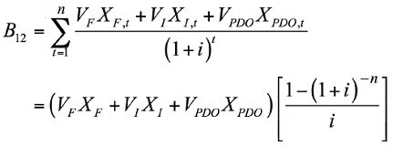
The value of safety improvements facilitated through automated traffic signal performance measures (B subscript 21) is equal to a summation of terms across all values of t from 1 to n. The term is a quotient. The numerator of the quotient is the summation of three products. The first product is (V subscript F) multiplied by (X subscript F,t). The second product is (V subscript I) multiplied by (X subscript I,t). The third product is (V subscript PDO) multiplied by (X subscript PDO,t). The denominator of the quotient is the quantity (1 plus i) raised to the power of t. The value of safety improvements facilitated through automated traffic signal performance measures (B subscript 21) is also equal to the product of two quantities. The first quantity is the summation of three products. The first product is (V subscript F) multiplied by (X subscript F). The second product is (V subscript I) multiplied by (X subscript I). The third product is (V subscript PDO) multiplied by (X subscript PDO). The second quantity is a quotient. The numerator of the quotient is 1 minus the quantity (1 plus i) raised to the power of negative n. The denominator of the quotient is i.
where VF, VI, and VPDO are the values associated with fatal, injury, and property-damage only crashes, respectively; and XF,t, XI,t, and XPDO,t are the corresponding numbers of prevented crashes of each associated type, for year t, summed from years 1 through n, with interest rate i. As before, the second term is presented where the reductions are assumed to be the same for each year, using the constant values XF, XI, and XPDO.
Equation 22
Example Application
Consider a hypothetical local agency interested in deploying ATSPMs on 40 intersections along five coordinated routes. This represents only part of the agency's overall network but it covers areas where the agency has the most operational concerns and may expand in the future.
An interest rate of 2 percent is used for the future costs and benefits in this example.
This agency has controllers that require a firmware upgrade to enable high-resolution data collection. Thus, the agency has a controller procurement cost C1 = $0, but will incur some labor cost for controller firmware upgrades. The assumption is made that no additional cost is required to obtain updated firmware. Assuming that all 40 intersections are affected, the average labor cost is $80/hour (h), and each intersection requires 4 h to accomplish the upgrade, then this cost works out to be, from equation 9:
Since this agency is not using external data collectors, cost C3 = $0. In this example it is further assumed the agency has existing communication systems that will permit data transfer; therefore, C4 = $0 and C5 = $0.
The agency has decided to add new detection to eight of its intersections to be able to measure vehicle arrivals; it is procuring these systems at a cost of $16,000 per intersection, yielding a total cost of $128,000. The agency attributes 50 percent of this cost to ATSPM deployment; thus, C6 = $64,000. Maintenance is anticipated to cost $1,000/yr over a 10-yr period; the net present value of this can be found using the second form of equation 8:
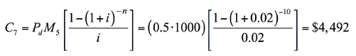
(C subscript 7) is equal to the product of (P subscript d), (M subscript 5), and a quotient. The numerator of the quotient is (M subscript 5,t). The numerator of the quotient is 1 minus the quantity (1 plus i) raised to the power of negative n. The denominator of the quotient is i. Therefore (C subscript 7) is equal to the product of 0.5, 1000, and a quotient. The numerator of the quotient is 1 minus the quantity (1 plus 0.02) raised to the power of negative 10. The denominator of the quotient is 0.02. Therefore (C subscript 7) is equal to $4,492.
Maintenance for the system (C7) is anticipated to cost $4,492 over a 10-yr period.
Most of the other existing detectors will need to be reconfigured to add detection zones for data-collection purposes. This is anticipated to require 3 hours per intersection. The labor cost is estimated at $80/h. According to equation 3 the total cost is:
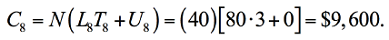
(C subscript 8) is equal to the product of N and a quantity. The quantity is equal to (U subscript 8) plus the product of (L subscript 8) and (T subscript 8). Therefore (C subscript 8) is equal to the product of 40 and a quantity. The quantity is equal to zero plus the product of 80 and 3. Therefore (C subscript 8) is equal to $9,600.
Detector documentation is expected to require 1 hour per intersection. Using equation 10, the cost is:
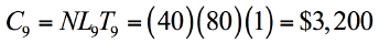
(C subscript 9) is equal to the product of N, (L subscript 9), and (T subscript 9). Therefore (C subscript 9) is equal to the product of 40, 80, and 1. Therefore (C subscript 9) is equal to $3,200.
The agency is procuring a new server at a cost of C10 = $24,000. Server maintenance is anticipated to require 40 hours per year (h/yr), or 400 h over a 10-yr period, with an average labor cost of $80/h. No annual fee is assumed to exist (F11 = 0). Each year, hardware replacements of $1,000 are anticipated. From equation 11, the server maintenance cost is:
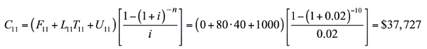
(C subscript 11) is equal to the product of two terms. The first term is the quantity of (F subscript 11) plus (U subscript 11) plus the product of (L subscript 11) and (T subscript 11). The second term is a quotient. The numerator of the quotient is 1 minus the quantity (1 plus i) raised to the power of negative n. The denominator of the quotient is i. Therefore the first term is the quantity of 0 plus 1000 plus the product of 80 and 40. And in the second term, the numerator of the quotient is 1 minus the quantity (1 plus 0.02) raised to the power of negative 10. The denominator of the quotient is 0.02. Therefore (C subscript 11) is equal to $37,727.
The agency has decided to use open-source ATSPM software, so its license cost is C12 = $0. However, it has hired a consultant to install and set up the system at a unit cost of $20,000. In addition, that work is anticipated to use 80 h of staff time at a labor cost of $35/h. From equation 13 the total cost of server setup is:

(C subscript 13) is equal to (U subscript 13) plus the product of (L subscript 13) and (T subscript 13). Therefore (C subscript 13) is equal to 20,000 plus the product of 80 and 80. Therefore (C subscript 13) is equal to $26,400.
Maintenance of the software is estimated to have similar requirements as server maintenance, about 40 h/yr (400 over a 10-yr period) at a cost of $80/h. No annual subscription fee is assumed to exist (A14 = 0). Using equation 14:
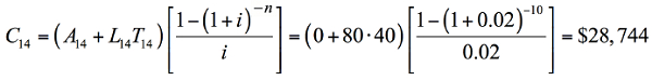
(C subscript 14) is equal to the product of two terms. The first term is the quantity of (A subscript 14) plus the product of (L subscript 14) and (T subscript 14). The second term is a quotient. The numerator of the quotient is 1 minus the quantity (1 plus i) raised to the power of negative n. The denominator of the quotient is i. Therefore the first term is the quantity of zero plus the product of 80 and 40. And in the second term, the numerator of the quotient is 1 minus the quantity (1 plus 0.02) raised to the power of negative 10. The denominator of the quotient is 0.02. Therefore (C subscript 14) is equal to $28,744.
For business process integration, the agency plans to invest 240 hours in training activities, at an average cost of $80/h, to bring agency capability to level 3 of the capability maturity framework. From equation 15:
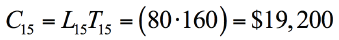
(C subscript 15) is equal to the product of (L subscript 15) and (T subscript 15). Therefore (C subscript 15) is equal to the product of 80 and 160. Therefore (C subscript 15) is equal to $19,200.
For usage of ATSPMs to achieve benefits, the agency estimates it will use 160 h/yr at an average cost of $80/h. From equation 16:
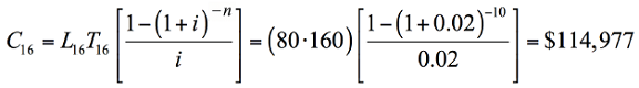
(C subscript 16) is equal to the product of two terms. The first term is the product of (L subscript 16) and (T subscript 16). The second term is a quotient. The numerator of the quotient is 1 minus the quantity (1 plus i) raised to the power of negative n. The denominator of the quotient is i. Therefore the first term is the product of 80 and 160. And in the second term, the numerator of the quotient is 1 minus the quantity (1 plus 0.02) raised to the power of negative 10. The denominator of the quotient is 0.02. Therefore (C subscript 16) is equal to $114,977.
The sum of these costs is $345,139.
On the benefit side, the reduction of labor for manual data collection represents a potential cost savings. For a fair comparison, the labor involved in this task could consider not only current data-collection practices, but could also reflect an increase in data collection needed to bring operations to the same level. In this example, the agency estimates that for its 40 intersections, collecting 16 hours of turning movement counts four times per year would require 2,560 h/yr. Manual data collection is estimated to cost $30/h as an estimated loaded rate for an entry-level worker. The agency estimates this activity can be completely eliminated using ATSPMs. Using equation 18:
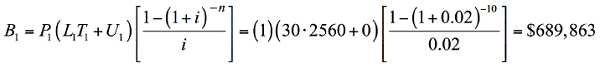
(B subscript 1) is equal to the product of three terms. The first term is (P subscript 1). The second term is the quantity of (U subscript 1) plus the product of (L subscript 1) and (T subscript 1). The third term is a quotient. The numerator of the quotient is 1 minus the quantity (1 plus i) raised to the power of negative n. The denominator of the quotient is i. Therefore the first term is equal to 1. The second term is the quantity of zero plus the product of 30 and 2560. And in the third term, the numerator of the quotient is 1 minus the quantity (1 plus 0.02) raised to the power of negative 10. The denominator of the quotient is 0.02. Therefore (B subscript 1) is equal to $689,863.
The agency estimates it spends about $500 per intersection per yr on preventative maintenance checks and scheduled retiming, which scales up to about $20,000/yr for 40 intersections. The agency believes it can reduce this level of effort by about 25 percent. Using equation 19, the benefit for this item is:
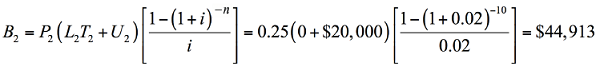
(B subscript 2) is equal to the product of three terms. The first term is (P subscript 2). The second term is the quantity of (U subscript 2) plus the product of (L subscript 2) and (T subscript 2). The third term is a quotient. The numerator of the quotient is 1 minus the quantity (1 plus i) raised to the power of negative n. The denominator of the quotient is i. Therefore the first term is 0.25. The second term is the quantity of zero plus the product of 500 and 40. And in the third term, the numerator of the quotient is 1 minus the quantity (1 plus 0.02) raised to the power of negative 10. The denominator of the quotient is 0.02. Therefore (B subscript 2) is equal to $44,913.
The agency estimates it spends an average of 2 hours per intersection per year responding to public complaint calls. This scales up to 800 hours over a 10-yr period. The average labor cost for this activity is estimated at $80/h. It expects this effort can be reduced by 50 percent. Using equation 20, the associated benefit is:
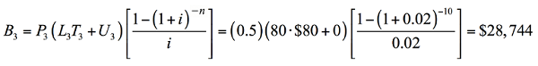
(B subscript 3) is equal to the product of three terms. The first term is (P subscript 3). The second term is the quantity of (U subscript 3) plus the product of (L subscript 3) and (T subscript 3). The third term is a quotient. The numerator of the quotient is 1 minus the quantity (1 plus i) raised to the power of negative n. The denominator of the quotient is i. Therefore the first term is 0.5. The second term is the quantity of zero plus the product of 80 and 80. And in the third term, the numerator of the quotient is 1 minus the quantity (1 plus 0.02) raised to the power of negative 10. The denominator of the quotient is 0.02. Therefore (B subscript 3) is equal to $28,744.
While acknowledging a benefit to possessing data for performance documentation, the agency decided not to include a monetary estimate of this benefit in its analysis, so B4 = $0.
Moving on to the public benefits described by B5–B11, the agency decided to include the short-term benefits by considering annualized benefits of the first year, and then estimating long-term benefits in similar terms. In its analysis, the agency has excluded benefits due to miscellaneous equipment failures, improved pedestrian service, and preemption issues, thus setting B7, B11, and B12 to $0. These were not considered major issues at the intersections under consideration.
For failed detection, the agency roughly estimated that 20 percent of all movements in its system, or 64 total, likely would be affected by detector failures in the short term; this would be equivalent to having one or more detector failures at eight intersections, affecting multiple movements. It assumed these would have lasted an average of 12 weeks. An average delay of 30 seconds was anticipated from these failures. Assuming that, on average, 200 vehicles per day per movement were affected, over a 12-week period this would lead to an average of 16,800 vehicles affected for each failure.
For the long-term analysis, the same 20 percent of movements experiencing 30 seconds of delay was retained. However, the time to discovery was assumed to be far less, so that only an average of 840 vehicles (5 percent of 16,800) would be affected, on average, for each failure. A value of $17.50/h was used for the value of time, and an average vehicle occupancy of 1.1 passengers per vehicle. The following brings these terms together using equation 21:
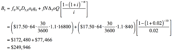
(B subscript 5) is equal to the summation of two quantities. The first quantity is the product of (f subscript 0), (N subscript 0), (D subscript k,0), (o subscript 0), and (q subscript 0). The second quantity is the product of two terms. The first term is the product of f, N, (? subscript k), o, and Q. The second term is a quotient. The numerator of the quotient is 1 minus the quantity (1 plus i) raised to the power of negative n. The denominator of the quotient is i. Therefore the first quantity is the product of 17.50, 64, 0.00833, 1.1, and 16,800. The first term of the second quantity is the product of 17.50, 64, 0.00833, 1.1, and 840. In the second term of the second quantity, the numerator of the quotient is 1 minus the quantity (1 plus 0.02) raised to the power of negative 10. The denominator of the quotient is 0.02. Therefore (B subscript 5) is equal to $249,946.
For failed communication, it was assumed that one corridor would lose communication within the first year that ordinarily would take about 12 weeks to respond to. Here it was also assumed that about 30 seconds of delay would be accumulated, affecting an average of 2,400 vehicles per day (veh/day), or 201,600 over the 12-week period. For the long-term analysis, the same terms were retained except that instead of 12 weeks, the failures were anticipated to be resolvable within 1 day, so that only 2,400 vehicles would be affected. Other terms remained the same as in B5:
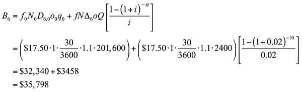
(B subscript 6) is equal to the summation of two quantities. The first quantity is the product of (f subscript 0), (N subscript 0), (D subscript k,0), (o subscript 0), and (q subscript 0). The second quantity is the product of two terms. The first term is the product of f, N, (? subscript k), o, and Q. The second term is a quotient. The numerator of the quotient is 1 minus the quantity (1 plus i) raised to the power of negative n. The denominator of the quotient is i. Therefore the first quantity is the product of 17.50, 1, 0.00833, 1.1, and 201,600. The first term of the second quantity is the product of 17.50, 1, 0.00833, 1.1, and 2,400. In the second term of the second quantity, the numerator of the quotient is 1 minus the quantity (1 plus 0.02) raised to the power of negative 10. The denominator of the quotient is 0.02. Therefore (B subscript 6) is equal to $35,798.
Benefits from improved capacity allocation were anticipated as affecting 80 movements; an average performance improvement of 10 seconds of delay was used, affecting an average of 400 veh/day. For the short-term benefit, this was annualized across weekdays: 400 × 5 × 52 = 104,000 vehicles affected per movement on average. For the long-term analysis, the same assumptions were made but delay improvements were estimated about 10 percent as large as the initial benefit, or 1 second on average. The other terms remained the same as in earlier analyses:
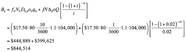
(B subscript 8) is equal to the summation of two quantities. The first quantity is the product of (f subscript 0), (N subscript 0), (D subscript k,0), (o subscript 0), and (q subscript 0). The second quantity is the product of two terms. The first term is the product of f, N, (? subscript k), o, and Q. The second term is a quotient. The numerator of the quotient is 1 minus the quantity (1 plus i) raised to the power of negative n. The denominator of the quotient is i. Therefore the first quantity is the product of 17.50, 80, 0.00278, 1.1, and 104,000. The first term of the second quantity is the product of 17.50, 1, 0.000278, 1.1, and 104,000. In the second term of the second quantity, the numerator of the quotient is 1 minus the quantity (1 plus 0.02) raised to the power of negative 10. The denominator of the quotient is 0.02. Therefore (B subscript 8) is equal to $844,514.
Finally, the benefit from improved progression was anticipated as affecting all five routes, with an average travel time reduction of 30 seconds affecting 2,400 veh/day. To annualize over the first year over 5 weekdays: 2,400 × 5 × 52 = 624,000 vehicles total. For the long-term analysis, these terms remained the same except that 10 percent of the initial benefit was assumed, or 3 seconds on average. Other terms in the formula were the same as earlier:
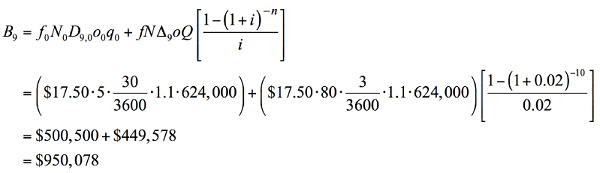
(B subscript 9) is equal to the summation of two quantities. The first quantity is the product of (f subscript 0), (N subscript 0), (D subscript k,0), (o subscript 0), and (q subscript 0). The second quantity is the product of two terms. The first term is the product of f, N, (? subscript k), o, and Q. The second term is a quotient. The numerator of the quotient is 1 minus the quantity (1 plus i) raised to the power of negative n. The denominator of the quotient is i. Therefore the first quantity is the product of 17.50, 5, 0.00833, 1.1, and 624,000. The first term of the second quantity is the product of 17.50, 80, 0.000833, 1.1, and 624,000. In the second term of the second quantity, the numerator of the quotient is 1 minus the quantity (1 plus 0.02) raised to the power of negative 10. The denominator of the quotient is 0.02. Therefore (B subscript 8) is equal to $950,078.
The total benefit from all of the above items is $2,843,856. In comparison with the cost of $345,139, this yields a total benefit-cost ratio of 8.2.
The above analysis is a very tentative example, with many introduced quantities that would require careful consideration from the agency. However, the overall analysis is intended to be as straightforward as the previous example. The previous analysis lands at resulting numbers similar in magnitude to those in previous field studies described earlier. In fact, this example is quite conservative regarding the overall benefit, given those studies focused on shorter time periods.
This example used an interest rate of 2 percent. Table 7 below shows how the results vary with different discount rates. As shown in table 7, the larger the interest rate, the smaller the net present values of benefits and costs and resulting benefit-cost ratios, since many upfront cost items do not recur in subsequent years.
Table 7. Effect of interest rates.
| Interest Rate (%) |
Total Cost ($) |
Total Benefit ($) |
Benefit-Cost Ratio |
| 0 |
365,530 |
3,035,855 |
8.30 |
| 1 |
355,011 |
2,936,003 |
8.27 |
| 2 |
345,139 |
2,843,856 |
8.24 |
| 3 |
336,001 |
2,758,561 |
8.21 |
| 4 |
327,531 |
2,679,501 |
8.18 |
| 5 |
319,670 |
2,606,126 |
8.15 |
Conclusions and Future Work
This chapter presented the preliminary vision for a methodology for calculating benefits and costs relative to ATSPM deployments. The methodology includes 16 potential cost items and 12 benefit items that can be considered by analysts. Each item is described and provided a basic formula for calculating using a set of relevant inputs. An example is applied to this methodology to yield a benefit-cost analysis for a hypothetical deployment.
A challenge in making this tool useful for agencies planning an ATSPM deployment will be in quantifying all elements in these formulas. At present, it is difficult to make recommendations on what the values should be, simply because there have only been a few previous studies that documented such outcomes. A further challenge is assigning quantitative value to benefits generally felt to be qualitative. An example presented here is the ability of ATSPMs to help agencies better communicate with decision makers and the public. The true value of this contribution may not easily be reduced to a number; it may be better reserved outside of a numerical analysis. Some costs are also not easily quantified; for example, shifting toward performance-based management involves a degree of cultural change in agency practices, which may involve more than training activities to overcome.