Road Weather Management Benefit Cost Analysis CompendiumCHAPTER 6. CASE STUDIES FOR DECISION SUPPORT, CONTROL, AND TREATMENT
Note: Use the hyperlinks in this table to jump directly to the case study.
CASE STUDY 6.1 — MINNESOTA DEPARTMENT OF TRANSPORTATION GATE OPERATIONS41
Project Technology or StrategyMNDOT developed an operational procedure known as freeway gate closure system for directing traffic off Interstates and prohibiting access during unsafe driving conditions such as severe snowstorms and major incidents. This procedure involves using gates both on the mainline to direct traffic off an Interstate and at entrance ramps to block traffic accessing an Interstate. While using gates is a relatively new technique for closing roadways to travel in Minnesota, neighboring States such as North and South Dakota have used gates for a number of years. During severe snowstorms and major incidents, mainline gates divert traffic from highways, and gates located on entrance ramps prohibit highway access. Generally, MNDOT personnel report to gate locations and activate warning signs with amber lights. Gate arms are then swung or lowered into place and gate arm lights are illuminated. Once gate arms are deployed, law enforcement personnel man gate locations for 1—2 hours. MNDOT's practice includes closing the Interstate to all traffic and prohibiting access to the Interstate when towns ahead cannot accommodate additional stranded vehicles. Project Goals and ObjectivesDuring a 1998 snow storm, MNDOT reduced roadway clearance costs by 18 percent on I-90 by activating a freeway gate closure system to limit vehicle interference and reduce snow compaction problems that increase work for plows. Between March and August 1999, MNDOT's Office of Advanced Transportation Systems conducted a BCA that compared potential savings to estimated costs to document past procedures and to identify current operational issues associated with gate systems. Gates were first used in Minnesota on Interstate 94 during the winter of 1996/97 and today 65 gates are used in three of MNDOT's eight Districts. In MNDOT District 4, 22 gates are used on portions of Interstate 94 and Highways 10 & 210, and in Districts 6 & 7, 43 gates are used on portions of Interstate I-90. As the use of gates has spread in Minnesota, MNDOT has become increasingly interested in documenting the experience to date with the gates and identifying any opportunities to enhance gate operations, particularly through the utilization of Intelligent Transportation Systems (ITS). As a result, MNDOT's Office of Advanced Transportation Systems (OATS) undertook this study to document past experience, identify issues and to recommend enhancements to the current operations. MNDOT hired the consulting firm of BRWM, Inc. to assist with the study that was conducted between March and August 1999. In order to provide comparable benefits and costs within the analysis, MNDOT carefully selected key MOEs to fully capture the benefits of the program. These measures included:
MethodologyThis benefit-cost analysis (BCA) for the proposed gate use on I-90 focuses on the cost of deployment along with the associated benefits due to savings in delays and reductions in accidents. The annual frequency of snow- and ice- related accidents and hourly volume data were used in the analysis. Total system costs were calculated assuming deployment costs of $159,700 plus 5 percent operations and maintenance costs over 10 years. COSTS Travel Delay Associated Costs. Table 22 presents the average delay and associated costs each year due to the closure of I-90 in MNDOT District 7. The analysis assumes one closure per year for a period of 3 hours affecting a percentage of Average Annual Daily Traffic (AADT). The AADT was calculated to be 8,000 (6,900 for passenger vehicles and 1,100 for heavy trucks) using values along I-90 from the 1994 MNDOT District 7 Trunk Highway Traffic Volume Map.
a Assumes one closure per year affecting 18 and 8 percent of trucks and 8 and 4 percent of cars for the high and low volume scenarios, respectively.
bThe values of time per hour were derived from the default values of MicroBENCOST, microcomputer based model developed by the Texas Transportation Institute at Texas A&M University. The default values were updated using the CPI. The value of time for heavy trucks is an average of values for different truck types. cThe average annual cost is calculated assuming a 3-hour delay. BENEFIT Travel Delay Cost Savings. Hourly distributions were obtained from Automatic Traffic Recorder (ATR) Data for 1994, Station 227 E&W, located east of Alden in Freeborn County. The high volume scenario assumes the closure occurs during the highest volume 3 hours of the day, from 3 p.m. to 6 p.m. with 22.6 percent of AADT. This calculates to 1,808 total vehicles delayed, with 550 assumed to be trucks. Assuming a certain minimum volume of traffic is required to justify closing the interstate, the hours of 6 a.m. to 9 a.m. with a volume of 10.4 percent AADT were used for the low volume scenario. This calculates to 832 total vehicles delayed, with 275 assumed to be trucks. The potential annual delay and accident cost savings as a result of deploying gates on I-90 are found in Table 23 and Table 24. Once again, a range is presented because it is not possible to pinpoint the actual reductions in delay and accidents that will occur due to the deployment of gates on I-90.
Accident Cost Savings. There are approximately 80 snow- and ice- related crashes per year on this segment of I-90. The average cost per accident is estimated to be $7,876. This assumes 81.38 percent of the accidents are property damage only with a total cost of $2,700 each, and 18.62 percent are personal injury with a total cost of $30,500 each. These accident costs are the values currently being used by MNDOT. The values are based on the average cost of accidents obtained from the four largest insurance carriers in Minnesota.
Model Run ResultsThe report documents potential savings attributed to a reduction in delays experienced by both passenger vehicles and heavy trucks. Based on AADT recorded by MNDOT in District 7, a delay of 3 hours on I-90 can cost between $36,400 during a low-volume period up to $78,000 during a high-volume period. In addition to a reduction in delays, cost estimates for a reduction in the number of accidents are also presented. Potential savings for accident reduction use an estimated average cost per accident calculated to be $7,900. This figure is based on values currently used by MNDOT to estimate accident costs. There are approximately 80 snow- and ice-related crashes per year on the segment of I-90 controlled by gates. A 5 percent reduction (4 accidents) in accidents annually will lead to an estimated annual savings of $31,504. These potential savings were compared with the estimated costs of gates. Based on information from District 7B, the cost for materials and installation of 43 gates averaged approximately $3,700 per gate. The potential ranges of benefit cost ratios published in the report are summarized in Table 25. Benefits outweighed the costs when the accident reduction is at least 3 percent for both low and high volumes and when the reduction in high-volume delay is 40 percent, even if there is no reduction in accidents.
Note: Discount rate = 5%
*The range of benefits goes from a low of $28,096 with a 10% reduction in delay in the low volume scenario and no reduction in accidents to $664,414 with a 70% reduction in delay in the high volume scenario and a 5% reduction in accidents. ** Assuming deployment costs of $159,700 +5% operations & maintenance costs over 10 year for 39 manually operated gates. Key ObservationsThis case showed that MNDOT and law enforcement personnel's gate closure projects are cost effective. After installing and using the gates, there is unanimous support for keeping the gates and enhancing how they are used. The gates provide a clear and indisputable notice that the road is closed and travel is prohibited. However, there is some frustration over roadways being closed when it appears the roadway is clear enough for traffic to make short trips between exits. When conducting a BCA, it is often useful to consider a range of alternatives and potential outcomes. This can provide insight into the project characteristics that drive either costs or benefits. In this analysis the authors show benefits associated with changes in assumed delay and accident rates. ReferenceBRW, Inc., Documentation and Assessment of MNDOT Gate Operations (Minnesota DOT: October 1999). Available at: http://www.dot.state.mn.us/guidestar/1996_2000/i90_i94_gate_closure/gatereport.pdf CASE STUDY 6.2 — HYPOTHETICAL ROAD CLOSURE FEASIBILITY42
Project Technology or StrategySevere winter weather makes travel unsafe and dramatically increases crash rates. Road closure strategies should allow users to avoid crash costs and eliminate costs associated with rescuing stranded motorists when conditions become unsafe due to winter weather. Some of the Snow Belt States recently gated entrances to physically close sections of rural freeways during severe winter storms. The benefits of efficient road closure strategies are the delay time savings and avoided safety costs. The costs of road closures are installation costs, operational costs, and some other costs, including the delays that are imposed on motorists and motor carriers who would have made the trip had the road not been closed. Project Goals and ObjectivesThe purpose of this hypothetical example is to examine the benefits and costs of winter weather road closure and develop a framework for their analysis. The benefit side of the analysis focuses on the safety issues related to road closures and the value of travel time. The cost of a road closure is concerned with infrastructure costs and operations and maintenance costs. MethodologyThe data used in this hypothetical scenario is similar to the data presented in the BCA on a gate closure system developed and published by Minnesota DOT (see Case Study 6.1). The analysis assumes one closure per year for a period of 3 hours affecting a percentage of average annual daily traffic (AADT). The AADT was calculated to be 8,000 (6,900 for passenger vehicles and 1,100 for heavy trucks) using values along the urban freeway from the 1994 State Trunk Highway Traffic Volume Map. The values of time per hour are available as default inputs in TOPS-BC. The default values were updated using an assumed 2.5 percent annual growth rate. The value of time for heavy trucks is an average of values for different truck types. The average annual cost is calculated assuming a 3-hour delay. As it is not possible to pinpoint the actual reductions in delay and accidents that will occur due to road closures, a range of hourly distributions is presented. The high volume scenario assumes the closure occurs during the highest volume 3 hours of the day, from 3 p.m. to 6 p.m. with 22.6 percent of AADT. This calculates to 1,808 total vehicles delayed, with 550 assumed to be trucks. Assuming a certain minimum volume of traffic is required to justify closing the interstate, the hours of 6 a.m. to 9 a.m. with a volume of 10.4 percent AADT were used for the low volume scenario. This calculates to 832 total vehicles delayed, 275 of which were assumed to be trucks. There are approximately 80 snow- and ice-related crashes per year on this segment of freeway. The average cost per accident is calculated to be $7,876. This assumes 81.38 percent of the accidents are property damage only with a total cost of $2,700 each, and 18.62 percent are personal injury with a total cost of $30,500 each. The values are based on the average cost of accidents obtained from the four largest insurance carriers in a typical mid-western State. The total cost assumes deployment costs of $159,700 plus 5 percent operations and maintenance costs over 10 years. Assuming deployment costs of $159,700 + 5 percent operations and maintenance costs for 39 manually operated gates. BENEFIT COST ANALYSIS A BCA can be used to determine whether to implement this type of road closure strategy. This section will describe how to run a BCA using TOPS-BC. In this case, we will use information from the previous study to run this analysis. In this hypothetical example, the user can utilize the TOPS-BC architecture to set up the BCA, to estimate annualized cost and benefits, to apply alternate discount rates, to estimate some benefits and to display the results. Since TOPS-BC does not now provide cost and benefit data unique to a RWM road closure application, the user must supply much of these data. The information can be collected from other DOTs that have implemented road closure programs or the data can be produced from engineering estimates. A search of the Federal Highway Administration (FHWA) Intelligent Transportation Systems (ITS) Database may provide much of this information. To set up TOPS-BC to conduct this analysis, the user will open the spreadsheet modeling tool to the start page (Figure 29) and click on "Estimate Life-Cycle Costs." Then, in the left hand column of the Cost Page (Figure 30), click on "Road Weather Management." Depending on the current version of TOPS-BC, you may or may not see any information on the costs of road closure systems. If no road closure costs are displayed, the user can input cost data from available information on the specific project or may locate information on the FHWA ITS Cost database. (http://www.itscosts.its.dot.gov/its/benecost.nsf/ByLink/CostDocs). 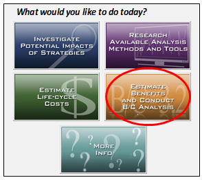 Figure 29. Screenshot. Tool for Operations Benefit/Cost start page - estimate benefits and conduct benefit cost analysis function. 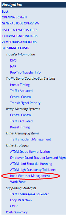 Figure 30. Screenshot. Tool for Operations Benefit/Cost navigation column for estimating costs - road weather management strategies. In addition to the characteristics that describe your project, such as technology-specific costs, roadway descriptions, number of installations, etc., you may also want to input values different from the TOPS-BC defaults for economic parameters related to the measure of benefits for the project. Examples may be the value of time or reliability. Others include the price of fuel, the cost of crashes, or the dollar value of other benefits. You may have data to support their inclusion; simply add the estimated value of these benefits to the "User Entered Benefit." Entering your own data allows you to make the analysis as specific as possible for your project. In addition, it provides a simple process for testing the sensitivity of the results to a particular variable or set of variables. In this case we have some specific site characteristics including length, number of lanes, and other characteristics. We also enter specific data about the performance of the facility, the value of reliability and the value of crash avoidance we are analyzing as TOPS-BC model doesn't provide default values for these parameters in the case of road weather management. Cost data inputs are located on the road weather management (RWM) cost sheet in TOPS-BC (Figure 31). We will modify the capital infrastructure equipment costs to reflect the installation of 39 closure gates. We have also added costs for incremental deployment equipment. However, we have shown there will be 0 incremental deployments, as for this analysis we are assuming that the 39 closure gates are installed concurrently and that the variable message signs and remote weather station are already in place. If they were not, then we would need to add costs for the incremental deployment of these systems. 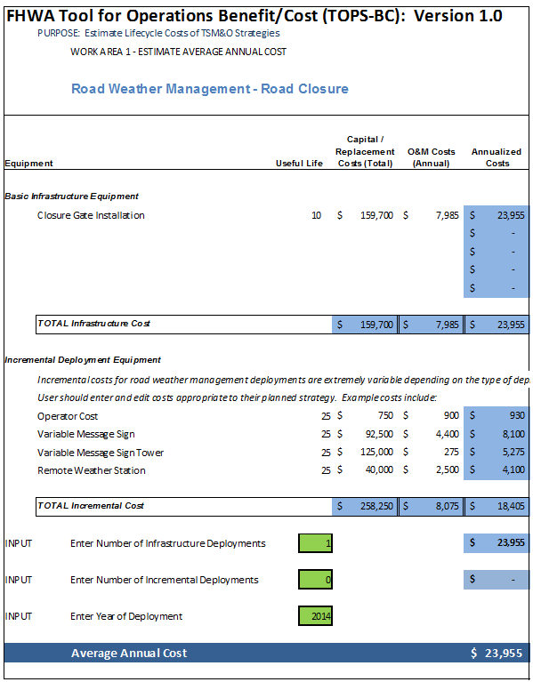 Figure 31. Screenshot. Cost estimate sheet from Tool for Operations Benefit/Cost for winter road closure analysis. Once the cost estimate is in place, return to the Navigation Column on the far left and click on the Benefit section for Road Weather Management (Figure 32). Here we will enter our safety data to complete the benefit side of the benefit cost ratio. For this case, we will assume that the number of injury crashes is reduced from 1 to zero and the number of property damage only crashes is reduced from 5 to zero (see red circles and arrows in Figure 33). 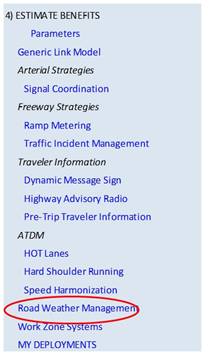 Figure 32. Screenshot. Tool for Operations Benefit/Cost navigation column for estimating benefits – road weather management strategies. 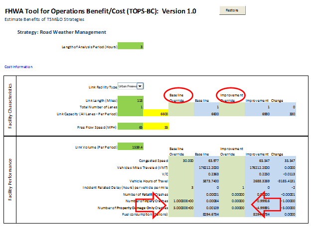 Figure 33. Screenshot. Benefit estimate sheet from Tool for Operations Benefit/Cost for winter road closure analysis. The user can also test the inputs to see where additional benefits may be realized. This can be accomplished by modifying assumptions about the project costs, size or other attributes. This gives the user a range of estimated benefits and costs. One can also test the value assumptions. For example, an alternative set of crash costs by type (fatality, injury or property damage) that only reflects local crash cost experience would improve the applicability of this tool for an individual project. 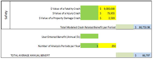 Figure 34. Screenshot. Benefit estimate sheet from Tool for Operations Benefit/Cost for winter road closure analysis (continued). Model Run ResultsTo view the results of the BCA, go to the left-hand navigation column and click My Deployments. The results are displayed in the middle of the page. They are reproduced in Figure 35. 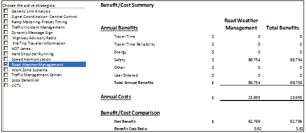 Figure 35. Benefit cost analysis summary sheet (partial) from Tool for Operations Benefit/Cost for winter road closure analysis. The TOPS-BC cost effectiveness analysis indicates that the average annual cost for this road closure policy will be $23,955 with total annual benefits from crash reductions are valued at $62,879. Other benefits for delay reduction, energy savings, maintenance crew deployment efficiencies, etc. would add to the total estimated benefits and would be included in the results display. Benefits. The primary benefits of road closure deployments are the reduction in crashes. The reduction in crashes provides a net annual benefit of about $62,879. Each project plan is different and the realized benefits can be impacted by the plan. By varying the assumptions in the plan, BCA models allow you to see how plan assumptions will impact the expected benefits. In this case, TOPS-BC estimates that the project benefits exceed the costs. This is a result of the reduction in crashes compared to the base case. As a result, we have increased the benefits provided to users per dollar of system costs. In economic parlance, we would say that the RWM investments and strategies evaluated would improve the operating efficiency for the system under study. Previous studies also demonstrated that with the freeway closed to travel there was less compaction due to vehicle travel, resulting in faster clearing times. Additionally, there were little or no stranded vehicles that interfered with State plowing operations on the freeway. Key ObservationsThis case discussed development of a TOPS-BC analysis model to test the feasibility of a road closure on rural interstate freeway in response to dangerous road weather conditions. Although this model is just a prototype, it provides a framework for the development of a tool that could be used to measure effectiveness in reducing delay times and safety costs (as measured by crash reductions), thereby providing an agency with objective and predictable measures for determining whether a closure is necessary. CASE STUDY 6.3 — HYPOTHETICAL FREEWAY SYSTEMS: DYNAMIC TRAFFIC SIGNAL CONTROL SYSTEMS DEPLOYMENT AND FEASIBILITY43
Project Technology or StrategyDynamic traffic signal (DTS) control involves placing a traffic signal linked to detectors at freeway onramps to regulate the flow of traffic entering the mainline facility and smoothing the flow of traffic during an inclement weather condition. DTS may be implemented with minimal cycle lengths, which simply break up platoons of vehicles entering the facility for an average day, or may be operated more aggressively with longer cycle lengths designed to function as gate regulators whose purpose is to maintain lower volumes on a freeway facility. DTS may be deployed at single isolated locations or region wide and are intended to improve road weather operations as a means of improving corridor travel times and safety. Similar to arterial signal systems, the sophistication of the timing patterns may be determined according to preset, traffic actuated, or centrally controlled patterns. Project Goals and ObjectivesIn this hypothetical scenario, a Midwestern traffic management agency wishes to deploy DTS on seven interchanges along a 5-mile corridor of a major interstate. The overall goal of the DTS program is to help decrease crashes and travel time delay while minimizing operational and management costs on freeway weather management. In this case we will use actual data from a previous study, but use the TOPS-BC tool to analyze the data. The objective of the case is to demonstrate the use of TOPS-BC to produce the project evaluation that is needed. MethodologyData is collected and analyzed prior to and after deployment of the DTS system to evaluate effectiveness. The data used for the analysis consists of loop detector speed and volume data and accident and incident management data. The study focuses on morning peak period (6 a.m. to 8 a.m.) and afternoon peak period (4 p.m. to 6 p.m.). This scenario assumes the 2010-2011 period for an initial evaluation. Historical data for a 24-month period prior to the implementation of the metering system will be used for the "before" period. The "after" period will use data collected over a 12-month period following the activation. For the Long Term Impacts Evaluation, we use archived data from morning and afternoon peak hours for the all no-holiday weekdays following the activation of the system. The results of the evaluation indicates that the DTS control systems will benefit traffic flow on the freeway and will meet or exceed the initially identified objectives for the system. BENEFIT COST ANALYSIS A BCA can be used to determine whether to implement DTS technology. TOPS-BC provides input defaults for most variables that would be used in the evaluation of a new DTS system. If a planner was looking at a system similar to this DTS example, he could use the TOPS-BC defaults or generate new data to make the example as realistic as possible by applying local data which can be applied in place of the defaults. This also allows the user to test the impact of changes in selected input data. For example, the analysis can be carried out for examples that highlight local or recent information for your project using different technology costs, traffic levels, wait times, etc. Each of the items shown in Table 26 are included in the default input data set, but may be replaced with user supplied data as shown. If user supplied data is entered, it will override the default value and be used by TOPS-BC in all calculations that call for that input data. In addition to the characteristics that describe your project, such as technology specific costs, roadway descriptions, number of installations, etc., you may also want to input values different from the TOPS-BC defaults for economic parameters related to the measures of benefits for the project. Examples may include the value of time or reliability, the price of fuel, the cost of crashes, or the dollar value of other benefits you may have calculated, such as vehicle emissions. TOPS-BC estimates fuel and emissions savings from VMT changes and assumptions about average fuel efficiency of the fleet. Some deployments may also reduce fuel consumption by changing the vehicle speed profile, but estimating this effect is beyond TOPS-BC. Entering your own data allows you to make the analysis as specific as you can for your project. In addition, it provides a simple process for testing the sensitivity of the results to a particular variable or set of variables. Table 26 illustrates both user-supplied data inputs and TOPS-BC-supplied inputs.
Note: User supplied inputs over ride TOPS-BC Supplied Input Defaults.
In this case we have some specific site characteristics including length, number of lanes, number of metered ramps, average speed, and other characteristics. We also enter specific data about the performance of the facility we are analyzing. TOPS-BC has already performed a literature review for the impacts of traffic-actuated road weather ITS and provides a consensus default value. However, in this case we have specific facility impacts and can input them into the system. We have chosen not to change the value of time, the value of reliability, energy prices, or the value of crash avoidance for this example. In this run we are accepting the TOPS-BC default values which can be found on the Parameters page in the TOPS-BC model.44 In this example, we are running TOPS-BC and we would like to modify the inputs to reflect new data. We might do this because of the similarity of this particular deployment to the one we are considering. We know that in this particular deployment, the freeway travel speeds increased by 20 percent and the number of crashes also decreased by 20 percent. However the TOPS-BC default for both these values was 12 percent. By using the navigation column we can go to the benefit inputs page and input the new percentage for speed and volume increases and crash reductions. These values will be used in all calculations calling for these values in TOPS-BC. The user can also test the inputs to see where additional benefits may be realized. This can be accomplished by modifying assumptions about the project costs, size, or other dimension. One can also test the value assumptions. For example, an alternative set of crash costs by type (fatality, injury or property damage only) that reflects local crash cost experience would improve the applicability of this tool for a specific project. The three primary benefits of DTS deployments are improvements in travel time, travel time reliability, and crashes. Each project plan is different, and the realized benefits can be impacted by the plan. By varying the assumptions in the plan, BCA models allow you to see how plan assumptions will impact the expected benefits. Travel Time. Travel time is usually calculated based on estimated link speeds in the corridor, both for the freeway and interstate links. Speeds may be estimated using the speed-flow relationship from the Highway Capacity Manual (HCM) where a speed factor (to be applied to free flow speed) for varying degrees of congestion (as measured by volume/capacity ratio) can be found. Speed is estimated for the baseline (without improvement) scenario by determining the correct speed-flow factor to apply based on your inputs for capacity and volume and applying the factor to the free flow speed you provided. These analyses must be performed separately for the freeway and interstate links. For the improvement scenario, average capacities are adjusted based on default impact percentages. BCA models usually provide these defaults, although the user can supply impact values if available. These default impact values are sensitive to the level of timing sophistication. The adjusted capacity value is used to determine an adjusted volume/capacity ratio which can be used to look up the speed-flow factor from the HCM or as a default in the model. The estimated speeds for the baseline and with improvement scenarios are used to estimate link travel time based on your inputs for link length and average volumes. The difference between the two scenarios in hours of travel time is monetized as the travel-time benefit. Travel Time Reliability. Travel time reliability can be based on the non-recurring delay estimation methodology developed for the second Strategic Highway Research Program (SHRP 2 projects L03 and L05). The approach uses factors (applied to VMT) representing the expected amount of incident-related delay based on the number of lanes on the facility, the length of the analysis period, the facility volume and the facility capacity. This analysis is only performed on the freeway links. The impact of the DTS strategy on incident-related delay is two-fold: it is impacted by both the change in facility capacity (discussed under the Travel Time impact above) as well as by a reduction in the number of crashes (discussed in the Crashes section below). The change in capacity results in a different volume/capacity ratio (between the without improvement and with improvement scenarios) being used with the incident related delay factors. The incident delay factor is multiplied by the VMT estimated for the facility. The resulting estimated number of hours of incident-related delay for the "with improvement" scenario are further reduced by the percentage decrease in the default crash rate. Additionally, according to the SHRP 2 research,45 the resulting recurring delay and incident delay values are applied in an additional algorithm along with the volume/capacity ratio to factor total non-recurring delay for the facility. The incremental change in hours of non-recurring travel time delay between the baseline and with improvement scenario is assigned a dollar value. Tools like TOPS-BC or similar models will do all these calculations for you with data you provide about your project and its expected effects on performance. Crashes. This data represents the benefit from the reduction in crashes that results from the smoothing of traffic conflicts in the merge area. A default crash rate factor is usually supplied by the BCA tool; however, if you have local data to support a different impact, you can usually input this project-specific information into your model. For example, with TOPS-BC you can enter a factor in the "Reduction in Freeway Crash Rate (%)" cell. This impact factor will reduce the crash rates applied to all crash severities. Dollar values will be applied to the change in the number of crashes to estimate this benefit. The reduction in the number of crashes is also fed back into the calculation of incident-related delay, producing a greater benefit level for travel time reliability. Other benefits are often associated with DTS strategies, including the reduction in vehicle emissions and fuel use beyond a change in travel demand. This is a change in vehicle efficiency caused by a change in vehicle operating profiles. These two benefits are inherently difficult to estimate within a spreadsheet-based model (e.g., spreadsheet-based models are generally incapable of estimating the vehicle acceleration and deceleration profiles to accurately assess these impacts). In TOPS-BC, you are free to modify the analysis framework to include these benefits, or simply to add the estimated value of these benefits to the "User Entered Benefit" cell if there is data to support their inclusion. Model Run ResultsThe TOPS-BC cost effectiveness analysis indicates that the first year cost for this DTS introduction will be will be $1.687 million with a continuing annual cost of $93,250 for a 20-year analysis period and with an additional cost every 5 years of $97,500 for software and system upgrades. This results in a 20 year net present value of just over $2 million, or a levelized annual cost of $172,600 with a 5 percent discount rate. If the deployment were already complete, we could then use the actual cost experience in this case if we believed it to be more accurate than the average cost shown by TOPS-BC. Note: Be cautious in overriding the default cost numbers. These values were developed from several reports on this technology and are thought to be accurate representations. Costs shown in a single report may not be comparable to the default values as they may not include all deployment costs. BENEFITS TOPS-BC estimates benefits from the DTS deployment from travel time savings, change in travel time reliability, reduced energy consumption, and reduced crash events. Together they result in levelized annual benefits of about $8 million. In this case, TOPS-BC estimates that the project benefits far exceed the costs. This results from the gain in operating efficiency for the system under study. TOPS-BC also estimated a substantial reduction in energy costs due to congestion relief. The number of crashes was also reduced, which provided the added benefit of crash-cost reduction.
Key ObservationsThis case identifies the introduction of a series of DTS control systems on an Interstate that is highly exposed to weather conditions. Prior to and after the deployment, the State DOT collected data on system performance to be able to compare the changes brought about by the deployment. Those performance changes revealed impacts on both freeway and DTS performance. These realized changes are what a pre-project deployment analysis needs in order to estimate the expected project benefits and costs. Once the project is deployed, performance indicators and their changes are known and can be used as an estimate of what might be expected if a similar project is deployed. CASE STUDY 6.4 — WEATHER RESPONSIVE SIGNAL TIMING (CONNECTED VEHICLE APPLICATION)46
Project Technology or StrategyWeather events can reduce the effectiveness of traffic signal timing plans and reduce arterial mobility. Several research studies found that in adverse weather average speeds declined by 16 percent to 40 percent, free-flow speed was reduced by 10 percent to 30 percent, traffic volumes were 15 percent to 30 percent lower, saturation flow rate fell by 2 percent to 21 percent, travel time delay increased by 11 percent to 50 percent, and there was 5 percent to 50 percent more start-up delay. Weather-related delays can be mitigated by implementing signal timing plans designed for slick pavement conditions and slower travel speeds. Investigations of traffic parameters sensitive to adverse weather assist analysts in developing weather-responsive traffic signal timing plans. Several of these benefit studies revealed that weather-responsive signal timing can improve arterial mobility by increasing average speed and reducing delay.47 Project Goals and ObjectivesRoad-weather connected vehicle data can be used to optimize signal timing for safety and mobility during adverse weather conditions. This means that high volume routes will have longer green phases. This technology can also be applied to ramp meters, with the reverse effect: ramp meters would allow a smaller number of cars on freeways and highways, because the risk of crashes decreases with lower traffic volume. Ramp meters can thus decrease delays on freeways during adverse weather conditions by controlling the entry volume and movement of traffic from the ramps. MethodologyCOSTS We used the information from the 2013 Road Weather Management Connected Vehicle Applications report48 to perform a benefit cost analysis (BCA) of the weather responsive signal timing application. Based on this data, new cost line items were added to the existing cost sheet within TOPS-BC.49 Figure 36 shows the different cost items that were added. The exhibit is taken from a spreadsheet within TOPS-BC that calculates the costs of specific CV strategies. Basic infrastructure refers to the required common infrastructure investments to support multiple CV transportation systems management and operations (TSMO) projects while the Incremental Deployment section includes cost items that are application-specific. The basic infrastructure and incremental deployment sections include estimated annualized costs, operations and maintenance costs, item-specific counts and the user-selected quantities used in this analysis. Since the case study CV deployments, including weather responsive signal timing, are assumed to take place in a hypothetical State, the distinction between necessary basic CV infrastructure investments and incremental/strategy-specific deployments needs to be clear. For the purpose of this analysis, each CV deployment BCA assumes that the respective State or metropolitan planning organization (MPO) needs to acquire both basic infrastructure and incremental/ strategy specific infrastructure. However, since the basic deployment investment supports many projects and strategies, only a portion of the total basic infrastructure cost is assigned to a specific CV technology. The percentage assumes that a set of CV technologies are deployed and the specific technology's basic infrastructure cost equals that technology's share of expected benefits in the set of deployed technologies. This cost assignment would vary depending on the full set of CV technologies deployed and supported by the basic infrastructure investment. For the weather responsive signal timing case study, the assumed percentage of total basic infrastructure costs is 26 percent. The 2013 CV report referenced above focused on the entire United States, so for the individual CV case studies in this compendium the hypothetical State is assumed to have 2 percent (1 of 50 States) of the total U.S. population. The basic infrastructure quantities used in the analysis were derived from that assumption and are shown in Figure 36. When the new cost items are entered into TOPS-BC, the 2013 CV report is used to identify which cost elements are needed to perform the appropriate cost analysis. If users want to analyze a specific connected vehicle application deployment strategy, the table allows for a quick identification of the cost items needed. 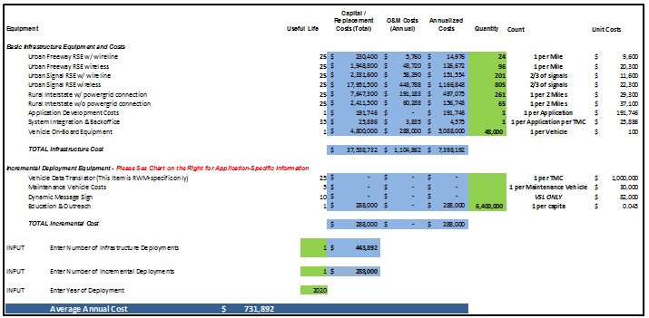 Figure 36. Screenshot. Annualized costs for weather responsive signal timing. This weather responsive signal timing application has several basic infrastructure cost items that need to be taken into consideration when conducting a BCA. These cost items are considered for this analysis and are listed below:
Additionally, there is one incremental cost item necessary for this CV application, education and outreach, which are necessary to inform the public about the implementation of the strategy. It is calculated on a per capita-basis, which means a cost occurs for every individual in the service area. Since the hypothetical State is assumed to have 2 percent of the U.S. population, this analysis uses the value of 6.4 million inhabitants, assuming that the U.S. population is 320 million. The following section focuses on the dollar values for basic infrastructure costs of a CV environment as well as the incremental cost item specific to this strategy. Figure 36 shows the annualized costs of this strategy as they were calculated using TOPS-BC. Finally, the number of infrastructure and incremental deployments was set to 1 each, because the extent of the roadway structure for the entire CV system and for this strategy in particular is already considered in the quantities shown in each cost line. The project is assumed to be in place in 2020. As Figure 36 shows, these assumptions result in annualized incremental costs of $731,892. BENEFITS In order to estimate the benefits of this strategy, we utilized the data from the CV BCA report which estimates the effectiveness of this strategy to be 7 percent. This means that crashes are likely to be reduced by 7 percent when the strategy is in place. Alongside this assumption is the assumed increase in capacity due to a lower amount of incidents that slow down traffic. The report set this number to 10 percent for all applications. Furthermore, crashes include three different types of incidents: property damage only, injury and fatality. Since TOPS-BC calculates the number of each of these types of incidents for all weather conditions and not just for adverse weather conditions, these values needed to be adjusted. For the purpose of this analysis, and based on the CV BCA report, it is assumed that 24 percent of incidents are related to adverse weather conditions. Hence this analysis applies to 24 percent of property damage only, injury, and fatality incidents. Figure 37 shows the CV benefit sheet within the tool. The adjusted values for property damage only, injury and fatality were entered into the green cells in the Facility Performance section of the tool. The green cells can be changed by the user and override the default values used by TOPS-BC. The capacity increase and crash reduction assumptions were implemented below the section Impacts due to Strategy. These values were also entered in the green cells, since TOPS-BC regularly does not consider any changes in capacity and uses a different crash reduction rate. For this reason, the given data within the tools were overridden. These data could come from travel demand models, freeway simulations, counts or other sources. Note that other agency benefits, such as benefits from reduced maintenance costs due to the weather responsive signal timing are not reflected in the benefit estimation. Analysts are encouraged to independently calculate such benefits and add them into the TOPS-BC estimates. 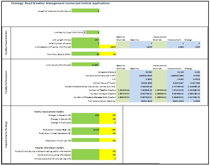 Figure 37. Screenshot. Benefit estimation assumptions for weather responsive signal timing. Finally, Figure 38 shows the lower half of the CV benefit estimation page. It includes additional sections on travel time, energy and other safety benefits. The user is able to refine any TOPS-BC calculation using these sections in case more specific data is at hand. Through this flexible user interface, the user can generate refined and more accurate results. The total average annual benefit is calculated automatically by TOPS-BC and can be found the bottom of the benefit estimation sheet. The total average annual benefit for this application is $13.32 million. 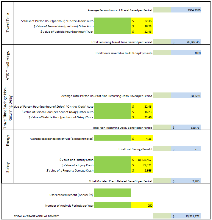 Figure 38. Screenshot. Benefit estimation results for weather responsive signal timing. There is limited data on the effectiveness of weather-responsive signal timing. The CV BCA report states that the number of incidents that occur in signalized intersections is about 6 percent of all crashes. The final benefits of this application are therefore estimated to be 6 percent of the total benefits of the application. The total benefits of this application are therefore 6 percent of the $13,321,771 shown in Figure 38, resulting in a total benefit of $799,306. Model Run ResultsFinally, the analysis compares the results of the benefits calculation with the results of the cost calculations. Note that this case study merely analyzes a specific set of costs and benefits for demonstration purposes. A full benefit cost analysis will include a wide range of additional costs and benefits that are not separately listed or analyzed in this case study. Figure 39 shows the section of TOPS-BC that compares benefits and costs for the connected vehicle strategy Weather Responsive Signal Timing. The exhibit indicates that the deployment of a Weather Responsive Signal Timing in a hypothetical State considering the underlying assumptions is cost effective, since the resulting BCR for the strategy is estimated at 1.09. The resulting net benefits for this analysis account for $67,417. 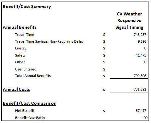 Figure 39. Screenshot. Results for weather responsive signal timing. CASE STUDY 6.5 — ROAD CONDITION REPORTING APPLICATION IN WYOMING50
Project Technology or StrategyThe recently completed weather responsive traffic management (WRTM) implementation project by the Wyoming DOT (WYDOT) included the development of a new mobile software application ("App") to improve the way maintenance staff report road conditions from the field. The App is used by WYDOT maintenance personnel to report road weather information to the traffic management center (TMC) it recommends variable speed limit changes, reports snow performance measures, and identifies a number of different traffic incidents including crashes and road hazards. Maintenance workers use the App, which was built to run on a tablet computer, to share information such as road conditions reported to the public, variable speed limits, weather information, messages posted on dynamic message signs, and map-based asset locations. The App can also be used to exchange email-type messages. The App was installed on 20 tablets, mostly in plow trucks. Project Goals and ObjectivesThe project goal was to develop a new software application to enhance the way maintenance personnel report road and weather conditions to headquarters and the traffic management center, recommend changes to variable speed limits, and report traffic incidents such as road hazards or crashes. Previously, these data were gathered manually and communicated via radio. The specific project objectives, which the App helped WYDOT to achieve, are to improve:
MethodologyThe evaluation of the condition reporting tool conducted by WYDOT and the Federal Highway Administration (FHWA) focused on quantitative and qualitative assessments of the changes in reporting and information processing related to road and traffic conditions. While the quantitative analysis primarily focused on comparing time spent by TMC operators to process such information, the qualitative analysis gathered data through two separate surveys: one completed by TMC operators and the other completed by maintenance employees.51 In general, the App improved the effectiveness and efficiency of road condition reporting and traffic management center activities during weather events. WYDOT plans to expand the App's usage during the winter of 2016 to as many as 150 vehicles. There was no benefit cost analysis (BCA) conducted as part of the project evaluation. The following analysis can serve as a hypothetical example of how BCA can be used to evaluate this type of project. The expanded version of TOPS-BC (Version 1.2 Beta for Connected Vehicles) developed by FHWA for demonstration purposes is used to analyze this case study, since the App developed by WYDOT can be evaluated like a connected vehicle application. COSTS For this case study, development costs for the WYDOT software application are estimated using data available in TOPS-BC. On the cost sheet for Version 1.2, the tool provides several cost line items separated into Basic Infrastructure Equipment and Costs and Incremental Deployment Equipment. The first section includes all costs that constitute basic infrastructure needs of an agency for all connected vehicle applications. Note that the information included in TOPS-BC is based on a study that estimated the benefits and costs of a nationwide connected vehicle deployment. Therefore, this case study only uses a fraction of the costs included in the tool. The second category includes all equipment items that are needed on an incremental basis; the size of the planned system determines the quantity of incremental equipment. For the cost estimation of the software application implemented by WYDOT, this analysis assumes significantly lower costs than the initial tool development for the nationwide study. These reduced costs are assumed for two reasons: (1) WYDOT already has technologies and procedures in place to acquire and report road weather conditions during adverse weather. It is unlikely that the full range of listed basic infrastructure and incremental costs in TOPS-BC was actually needed for this project, and (2) the information in TOPS-BC is based on a paper which performed a BCA of nationwide connected vehicle deployment. In contrast, this case study focuses on a software application deployment. It is reasonable to assume that this project does not require as extensive investments as the national estimate. Since these costs are unknown, this case study utilized a selected percentage of the standard Application Development Costs that is included as a cost line item within TOPS-BC. Figure 40 shows the cost page within the tool, the different line items of Basic Infrastructure Equipment and Incremental Deployment Equipment, as well as the total assumed costs for this strategy. The standard Application Development Costs within the tool for national deployment are $10,000,000. For this case study it is assumed that only a small percentage (0.25 percent) of that amount applies to the WYDOT road condition reporting app. This results in annual costs of $25,000. Furthermore this cost estimation considers on-board equipment (OBE) for 20 vehicles as mentioned in the introduction, amounting to additional $2,120. The total average annual costs for this project thus are $27,120. 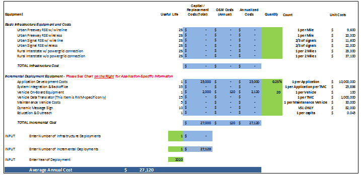 Figure 40. Screenshot. Wyoming road condition reporting application cost estimation sheet and results as displayed within the Tool for Operations Benefit/Cost. BENEFITS As resulting benefits of this strategy, significant TMC operator time savings were calculated from the automation of several key tasks — data logging and traveler information system updates. Based on road reports including storm days and non-storm days from January 2014 to December 2014, WYDOT estimates that using the App can result in more than one person-year of time savings for agency staff.52 This analysis assumes the monetized amount of one person-year to be an average salary of $60,000 annually. This amount is counted as an agency benefit, because, based on the source, the agency can save one person-year of time savings. Finally, this analysis also accounts for 20 percent of the annual salary for possible fringe benefits related to this person-year of staff savings. This case study demonstrates the process for estimating costs and benefits and performing a BCA using TOPS-BC for connected vehicle strategies. It does not consider a range of other benefits potentially applicable to this strategy, such as safety benefits, travel time savings, travel time reliability benefits, or other agency efficiency gains. If the user wants to perform a comprehensive BCA of this particular road weather management strategy or a related strategy, it is essential to include the benefits mentioned above, which are not considered explicitly in this case study. TOPS-BC allows the analyst to input unique, user-specific annual benefits on its benefit sheets. This feature was utilized for this analysis, since the monetary amount of benefits is mainly based on a national estimate. As a last step, $60,000 is multiplied by 1.2 in order to account for the 20 percent of assumed fringe benefits, resulting in a total of $72,000 of average annual benefits. Model Run ResultsFigure 41 shows the benefit/cost summary of the WYDOT Road Condition Reporting Application using TOPS-BC. Since the benefit estimation is based on national connected vehicle deployment estimates, there are only user entered benefits to be considered for this analysis. The costs of this project only represent a fraction of its benefits, since total costs are $27,120 compared to $72,000 of benefits for each year of deployment. These results generate a benefit-cost ratio of 2.65, as the exhibit indicates. Additional benefits associated with this strategy and the resulting improved traveler information, traffic management and maintenance operations are not included in the analysis. 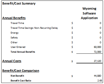 Figure 41. Screenshot. Benefit-cost analysis results for the Wyoming road condition reporting application as displayed within the Tool for Operations Benefit/Cost. Key ObservationsThis case study serves to demonstrate how TOPS-BC can be used to analyze improvements in road reporting systems. Users are encouraged to improve any assumptions utilized in this analysis based on their own region-specific data and other available databases. Through this effort, the results generated by TOPS-BC become more refined as more data is fed into the tool. More detailed and in-depth analyses of such a procedure may result in different benefit-cost ratios and net benefits. The tool offers various features that support such analyses, and its results can give the user a first impression on the cost efficiency of agency procedure and traffic improvement strategies. ReferencesFederal Highway Administration, Wyoming Department of Transportation (WYDOT) Road Condition Reporting Application for Weather Responsive Traffic Management, Final Report, US DOT, FHWA-JPO-16-266, October 2015. CASE STUDY 6.6 — WEATHER RESPONSIVE ACTIVE TRAFFIC MANAGEMENT SYSTEM IN OREGON53
Project Technology or StrategyOregon DOT (ODOT) has avoided spending nearly $1 billion on capacity and interchange improvements by implementing a weather responsive active traffic management system on State Route 217 (OR217), a 7.5 mile limited access highway in Portland, Oregon. ODOT designed and implemented various cost-saving active traffic management (ATM) strategies to improve safety, reliability, and mobility. The ATM system includes a comprehensive application of automated technologies to improve operations and safety on the corridor.54 The system manages traffic dynamically based on prevailing roadway conditions using integrated monitoring systems and coordinated responses. The project consisted of six interrelated systems: queue warning, congestion responsive variable speed, weather responsive variable speed, dynamic ramp-metering, travel time information, and curve warning. Key facets of the project included advisory speeds based on weather and traffic conditions, variable message signs on the sides of roadways and surface streets providing real-time travel time estimates, and queue warnings. In addition, it involved targeted shoulder use and shoulder widening to provide space for impaired vehicles and to improve emergency vehicle access. Project Goals and ObjectivesThe project goals are to improve highway efficiency and safety as long-term solutions, avoiding high-cost investments of major construction by employing relatively low-cost ATM solutions. Oregon Route 217 is a heavily trafficked 7.5-mile limited access highway that runs north-south through the cities of Beaverton and Tigard between Interstate 5 and US 26. The roadway frequently operates at high capacity levels as traffic has more than doubled in the past thirty years, resulting in significantly decreased safety and reliability.55 While studies have recommended capacity and interchange improvements costing nearly $1 billion, such as widening to six lanes, braiding ramps, and adding collector-distributor roadways, ODOT opted for the development of more cost-effective ATM improvements. The changes are designed to:
MethodologyIn order to estimate the costs and benefits of the ATM system in Oregon, we utilized the Tool for Operations Benefit Cost Analysis (TOPS-BC).57 This case study mainly serves to demonstrate the possibility for analyzing Active Transportation and Demand Management (ATDM) strategies deployed by ODOT to improve the traffic conditions on OR217. For this case study, we chose to analyze one of the six strategies deployed on the corridor, namely weather-responsive variable speed limits. FHWA expanded TOPS-BC to Version 1.2, which includes an analysis sheet for variable speed limits along various types of operational strategies. This Oregon case study uses that version. COSTS The costs of Oregon's weather responsive variable speed limits (VSL) project were estimated using the TOPS-BC cost sheet, which includes numerous line items that are unique to VSL. There are a number of default values for an initial VSL deployment within TOPS-BC, which are utilized for this cost estimation. Figure 42 shows the different cost items as they are listed within the tool. The costs are separated into two groups. The first is basic infrastructure equipment costs, which represent basic infrastructure investments necessary for the strategy. The second cost section, incremental deployment equipment costs, represents cost items associated with how extensively the system will be deployed. The quantities for this section were removed, since ODOT provided cost information on the total costs of the project as well as annual operations and maintenance (O&M) costs. The cost columns show annualized capital and O&M costs in three different columns, indicating that the tool can apply different cost values if needed. ODOT estimated the total costs for the ATM system at $8 to $10 million, so for this analysis we assumed a total cost of $9 million. Additional costs for the weather related VSL system are estimated to be $500,000. These two figures were combined in order to represent the project's total capital costs and then annualized over the average lifetime of the equipment, which is 25 years. Finally, ODOT estimated the O&M costs for the implemented system to be $50,000 annually. This amount was added to the previously tabulated annualized costs. 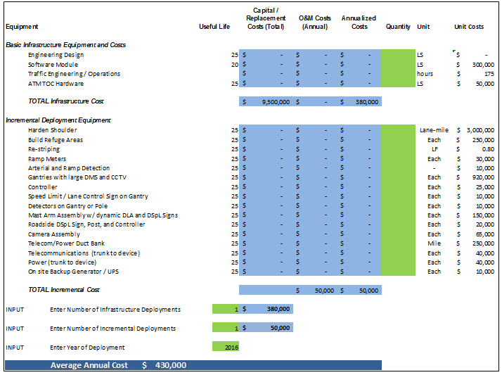 Figure 42. Screenshot. Cost estimation sheet in the Tool for Operations Benefit/Cost for the Oregon weather responsive active traffic management system. The bottom of the cost sheet shows the number of infrastructure and incremental deployments, which depend on the extent of the VSL system. Since the VSL system was implemented only on OR 217, the number of infrastructure and incremental deployments was set to 1 each. Finally, the cost sheet shows an average annual cost of about $555,000 for the VSL deployment. BENEFITS This section describes the benefit estimation for the weather responsive VSL deployment. We made several assumptions for the benefit estimation. Figure 43 shows an extract from the VSL Benefit Estimation sheet within the Beta Version 1.2 of TOPS-BC and includes these default assumptions. Since the focus of TOPS-BC is on peak periods as opposed to the entire day, the length of the analysis period is set to three hours, as this constitutes a standard peak period in a metropolitan area. Subsequently, the link facility type is set to Type 2 – Urban Freeway. The total length of the link in the case study is 7.5 miles, based on information from Oregon DOT. The average number of lanes is set to 2.5; this is because the number of lanes on OR217 is 2, but auxiliary lanes are put in place between interchanges, which is why this analysis assumes half the capacity for the auxiliary lanes. The link capacity in the yellow cell is calculated by the tool based on the number of lanes, length of the analysis period, and the link facility type. Free flow speed is set to 60 instead of the standard value of 55, because the analysis assumes that the average roadway user exceeds the official speed limit on a regular basis and ODOT provided similar information for this analysis. Finally, the link volume is set to 15,675 vehicles per period, analyzed in this write up. 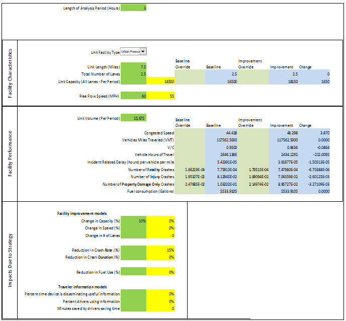 Figure 43. Screenshot. Benefit estimation assumptions for the Oregon weather responsive active traffic management system. The results of benefit and cost estimations are collected by TOPS-BC which is derived by calculating 95 percent of the link capacity. This assumption ensures that the traffic flow is heavy and close to the maximum capacity of the roadway structure for the peak period. Traffic demand management (TDM) simulations or counts, if available, could be substituted for the flow estimate. The crash values shown in the Facility Performance section include three different types of incidents: property damage only, injury, and fatality. TOPS-BC calculates the number of each incident type for all weather conditions, not just for adverse weather conditions. However, because the system being analyzed in Oregon is weather-responsive, these values had to be adjusted. Additional benefits could occur from the use of the other strategies mentioned earlier, but are not estimated here. For the purpose of this analysis, and based on a report by FHWA, it is assumed that 24 percent of incidents are related to adverse weather conditions.58 Hence this analysis applies to 24 percent of property damage only, injury, and fatality incidents. Finally, as a result of the implementation of all strategies in the ODOT ATM project, the assumption was made that these measures are going to free up 10 percent of additional capacity throughout peak periods. This is why the value of Change in Capacity in the Impacts due to Strategy section was set to 10 percent. Figure 43 shows the assumptions discussed above and gives an overview of what a benefit sheet within TOPS-BC looks like. Model Run ResultsThis section summarizes the results of the BCA of the VSL project. Please note that this case study merely analyzes a specific set of costs and benefits for demonstration purposes. A full BCA will include a wide range of additional costs and benefits that are not separately listed or on a single page within the tool. This gives the user a concise overview of the all estimations and their results. This sheet is called Summary of my Deployments and provides a benefit-cost summary. Figure 44 shows the benefit/cost summary for the weather responsive variable speed limit deployment in Oregon. Note that the heading states Active Transportation and Demand Management (ATDM), because VSL falls into this category of traffic management and operations measures. As the exhibit shows, the benefits exceed the costs of this strategy alone, without considering the other 5 ATDM strategies associated with the project. The BCA results in net benefits of about $1.52 million and a benefit-cost ratio of 4.54. A more complete analysis would include all costs and benefits of the full Oregon DOT ATM deployment strategies on OR217. 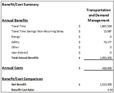 Figure 44. Screenshot. Benefit-cost analysis results for the Oregon weather responsive active traffic management system. ReferencesOregon Department of Transportation, OR217: Active Traffic Management (2015). Available at: http://www.nascio.org/portals/0/awards/nominations2015/2015/2015OR6-Oregon-ODOT-2015%20-%20OR217%20ATM%20Project.pdf FHWA, Road Weather Connected Vehicle Applications (2013), available at https://ntl.bts.gov/lib/54000/54400/54480/Road_Weather_Connected_Vehicle_Applications_Benefit-508-v8.pdf ITS 2015 award nomination package, submitted by D. Mitchell, Regional Traffic Engineer (ODOT). "OR 217: Active Traffic Management," for the Best New Innovative Product, Service, or Application category. CASE STUDY 6.7 — VARIABLE SPEED LIMIT (CONNECTED VEHICLE APPLICATION)59
Project Technology or StrategyThe vision of intelligent vehicles has generated numerous concepts to control future traffic flow, one of which is the in-vehicle actuation of traffic control signals. Key to this concept is the use of intelligent vehicles as actuators for traffic control systems, replacing the traditional roadside systems. Traffic speeds are regulated through variable speed limit (VSL) gantries to resolve stop-and-go waves, while intelligent vehicles control accelerations to optimize their local driving situation specifically. In this scenario, each intelligent vehicle receives VSL commands from the traffic controller and implements them into its driving behavior. Simulations show that the connected VSL and vehicle control systems improve traffic efficiency and sustainability; for example, total time spent in the network and the average fuel consumption rate are reduced compared to scenarios with 100 percent human drivers and to scenarios with the same intelligent vehicle rates.60 Project Goals and ObjectivesThis case study shows how road-weather connected vehicle data can be used to activate VSL systems to provide real-time information on appropriate speeds for current conditions, as well as warn drivers of impending road weather events. MethodologyCOSTS We used the information from the 2013 Road Weather Management Connected Vehicle Applications report61 to perform a benefit cost analysis (BCA) of the VSL application. Based on this data, new cost line items were added to the existing cost sheet within TOPS-BC.62 Figure 45 shows the different cost items that were added. The exhibit is taken from a spreadsheet within TOPS-BC that calculates the costs of specific CV strategies. Basic Infrastructure refers to the required common infrastructure investments to support multiple CV transportation system management and operations (TSMO) projects while the Incremental Deployment section includes cost items that are application-specific. The basic infrastructure and incremental deployment sections include estimated annualized costs, operations and maintenance costs, item-specific counts and the user-selected quantities used in this analysis. 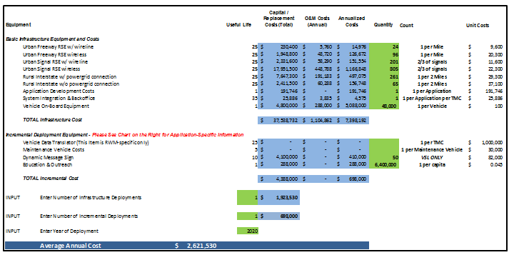 Figure 45. Screenshot. Annualized costs for variable speed limits for weather-responsive traffic management. Figure 45. Screenshot. Annualized costs for variable speed limits for weather-responsive traffic management.
Since the case study CV deployments, including VSL, are assumed to take place in a hypothetical State, the distinction between necessary basic CV infrastructure investments and incremental or strategy-specific deployments needs to be clear. For the purpose of this analysis, each CV deployment BCA assumes that the respective State or metropolitan planning organization (MPO) needs to acquire both basic infrastructure and incremental or strategy-specific infrastructure. However, since the basic deployment investment supports many projects and strategies, only a portion of the total basic infrastructure cost is assigned to a specific CV technology. The percentage assumes that a set of CV technologies are deployed and the specific technology's basic infrastructure cost equals that technology's share of expected benefits in the set of deployed technologies. This cost assignment would vary depending on the full set of CV technologies deployed and supported by the basic infrastructure investment. For the VSL case study, the assumed percentage of total basic infrastructure costs is 26 percent. The CV BCA report focused on the entire United States so for the individual CV case studies in this compendium the hypothetical State is assumed to have 2 percent (1 of 50 States) of the total U.S. population. The basic infrastructure quantities used in the analysis were derived from that assumption and are shown in Figure 45. When the new cost items are entered into TOPS-BC, the CV BCA report is used to identify which cost elements are needed to perform the appropriate cost analysis. If users want to analyze a specific connected vehicle application deployment strategy, the table allows for a quick identification of the cost items needed. As illustrated in Figure 45, this CV application has several cost items that need to be taken into consideration when conducting a BCA. The following cost items were included in this case study:
Figure 45 shows the cost sheet within TOPS-BC for this application. In addition to the basic infrastructure cost items mentioned above, the figure also shows quantities and dollar values for two cost items that are specific for this strategy:
Variable speed limit signs are necessary, since the speed limit will change depending on the weather and traffic conditions. For the hypothetical State, it is assumed that a total of 50 variable speed limit signs will be necessary throughout the network. Education and outreach are necessary to inform the public about the implementation of the strategy. It is calculated on a per capita-basis, which means a cost occurs for every individual in the service area. Since the hypothetical State is assumed to have 2 percent of the U.S. population, this analysis uses the value of 6.4 million inhabitants, assuming that the U.S. population is 320 million. Finally, the number of infrastructure and incremental deployments were each set to 1, because the extents of the roadway structure for the entire CV system and for this particular strategy area already considered in the quantities shown in every cost line. The VSL system is assumed to be operational in 2020. As Figure 45 shows, these assumptions result in annualized costs of about $2.62 million. BENEFITS In order to estimate the benefits of VSL strategy, we utilized again the data from the CV BCA report. According to these data, the effectiveness of this strategy is estimated to be 2 percent in the summer and 13 percent in the winter. This means that crashes are likely to be reduced by 2 percent and 13 percent in summer and winter respectively when the strategy is in place. Alongside this assumption is the assumed increase in capacity due to a lower amount of incidents that slow down traffic. The report set this number to 10 percent for all applications. Furthermore, crashes include three different types of incidents: property damage only, injury and fatality. Since TOPS-BC calculates the number of each of these types of incidents for all weather conditions and not just for adverse weather conditions, these values needed to be adjusted. For the purpose of this analysis, and based on the CV BCA report, it is assumed that 24 percent of incidents are related to adverse weather conditions. Hence this analysis applies to 24 percent of property damage only, injury, and fatality incidents. TOPS-BC is a sketch-planning level tool that calculates one distinct set of assumptions at a time. Since the levels of effectiveness vary between summer (2 percent) and winter (13 percent), the model is run twice for this application. Figure 46 shows the CV benefit sheet within the tool and the set of assumptions for this case study, including the rate of effectiveness for the summer. There is no specific figure included in this case study showing the winter rate of effectiveness, since the 2 percent value in Figure 46 was merely changed to 13 percent. Adjusted property damage only, injury and fatality values were input into the green cells in the Facility Performance section of the tool. The user can change the green cells and override the values calculated by TOPS-BC. The capacity increase and crash reduction assumptions were used below the section Impacts due to Strategy. These values were also used in the green cells, since TOPS-BC regularly does not consider any changes in capacity and uses a different crash reduction rate. For this reason, the given data within the tools were overridden. Finally, Figure 47 shows the lower half of the CV benefit estimation page for the summer assumptions. It includes additional sections on travel time, energy and other safety benefits. The user is able to refine any TOPS-BC calculation using these sections in case more specific data is available. Through this flexible user interface, the user can generate more refined and accurate results. The total average annual benefit is calculated automatically by TOPS-BC and can be found at the bottom of the benefit estimation sheet. The total annual benefit for this summer application is $13.2 million. The winter application yields an annual benefit of $13.52 million. For this case study, the average between these two numbers is used. The average annualized benefit for this application is $13.37 million. 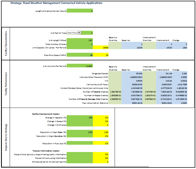 Figure 46. Screenshot. Benefit estimation assumptions for variable speed limits for weather-responsive traffic management (summer season). 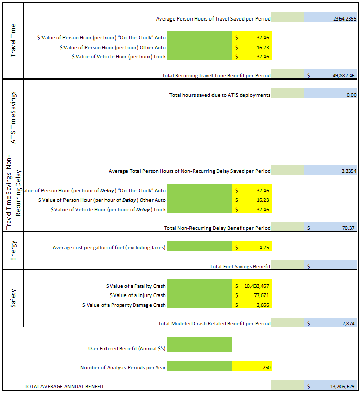 Figure 47. Screenshot. Benefit estimation result for variable speed limits for weather-responsive traffic management. Model Run ResultsFinally, the analysis compares the benefits calculation with the cost calculations. This case study merely analyzes a specific set of costs and benefits for demonstration purposes. A full benefit cost analysis will include a wide range of additional costs and benefits that are not separately listed or analyzed in this case study, such as environmental benefits, energy savings, and vehicle operating cost reductions. Figure 48 shows the section of TOPS-BC that compares benefits and costs for the CV variable speed limit strategy. The exhibit indicates that the deployment of a variable speed limit in a hypothetical State, all assumptions considered, is cost effective, since the resulting BCR for the strategy is 5.04. The resulting net benefits for this analysis are about $10.59 million. 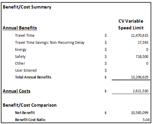 Figure 48. Screenshot. Results for connected vehicle variable speed limit strategy. 41 Chapters 2 and 3 of this Compendium contain a discussion of the fundamentals of BCAs and an introduction to BCA modeling tools. These sections also contain additional BCA references. [ Return to note 41. ] 42 Ibid. [ Return to note 42. ] 43 Ibid. [ Return to note 43. ] 44 For more information on modifying the TOPS-BC Parameters page, see case 7-10. [ Return to note 44. ] 45 See for example: http://www.trb.org/StrategicHighwayResearchProgram2SHRP2/Pages/Reliability_Projects_302.aspx [ Return to note 45. ] 46 Chapters 2 and 3 of this Compendium contain a discussion of the fundamentals of BCAs and an introduction to BCA modeling tools. These sections also contain additional BCA references. [ Return to note 46. ] 47 Lynette C. Goodwin and Paul A. Pisano, "Weather-Responsive Traffic Signal Control," ITE Journal, June 2004. [ Return to note 47. ] 48 FHWA, Road Weather Management Connected Vehicle Applications, available at https://ntl.bts.gov/lib/54000/54400/54480/Road_Weather_Connected_Vehicle_Applications_Benefit-508-v8.pdf [ Return to note 48. ] 49 FHWA, Tool for Operations Benefit/Cost Analysis, available at https://ops.fhwa.dot.gov/plan4ops/topsbctool/index.htm [ Return to note 49. ] 50 Chapters 2 and 3 of this Compendium contain a discussion of the fundamentals of BCAs and an introduction to BCA modeling tools. These sections also contain additional BCA references. [ Return to note 50. ] 51 FHWA, Wyoming Department of Transportation (WYDOT) Road Condition Reporting Application for Weather Responsive Traffic Management, FHWA-JPO-16-26 (Washington, DC: 2015), p. 27. Available at: https://ntl.bts.gov/lib/56000/56800/56890/FHWA-JPO-16-266_v2.pdf [ Return to note 51. ] 52 Ibid. [ Return to note 52. ] 53 Chapters 2 and 3 of this Compendium contain a discussion of the fundamentals of BCAs and an introduction to BCA modeling tools. These sections also contain additional BCA references. [ Return to note 53. ] 54 Oregon Department of Transportation, OR217: Active Traffic Management (2015). Available at: http://www.nascio.org/portals/0/awards/nominations2015/2015/2015OR6-Oregon-ODOT-2015%20-%20OR217%20ATM%20Project.pdf. [ Return to note 54. ] 55 Ibid, p.3. [ Return to note 55. ] 56 ITS 2015 award nomination package, submitted by D. Mitchell, Regional Traffic Engineer (ODOT): "OR 217: Active Traffic Management," for the Best New Innovative Product, Service, or Application category. [ Return to note 56. ] 57 FHWA, Tool for Operations Benefit/Cost Analysis, available at: https://ops.fhwa.dot.gov/plan4ops/topsbctool/index.htm [ Return to note 57. ] 58 FHWA, Road Weather Connected Vehicle Applications (2013), available at https://ntl.bts.gov/lib/54000/54400/54480/Road_Weather_Connected_Vehicle_Applications_Benefit-508-v8.pdf [ Return to note 58. ] 59 Chapters 2 and 3 of this Compendium contain a discussion of the fundamentals of BCAs and an introduction to BCA modeling tools. These sections also contain additional BCA references. [ Return to note 59. ] 60 Wang, Daamen, Hoogendoorn, van Arem, "Connected Variable Speed Limits Control and Vehicle Acceleration Control to Resolve Moving Jams," presented to the 94th Annual Meeting of Transportation Research Board, in Washington, D.C., January 2015. Available at: https://www.researchgate.net/publication/270892960_Connected_variable_speed_limits_control_and_vehicle_acceleration_control_to_resolve_moving_jams [ Return to note 60. ] 61 FHWA, Road Weather Management Connected Vehicle Applications, FHWA-JPO-14-124. Available at https://ntl.bts.gov/lib/54000/54400/54480/Road_Weather_Connected_Vehicle_Applications_Benefit-508-v8.pdf [ Return to note 61. ] 62 FHWA, Tool for Operations Benefit/Cost Analysis, available at https://ops.fhwa.dot.gov/plan4ops/topsbctool/index.htm [ Return to note 62. ] | |||||||||||||||||||||||||||||||||||||||||||||||||||||||||||||||||||||||||||||||||||||||||||||||||||||||||||||||||||||||||||||||||||||||||||||||||||||||||||||||||||||||||||||||||||||||||||||||||||||||||||||||||||||||||||||||||||||||||||||||||||||||||||||||||||||||||||||||||||||||||||||||||||||||||||||||||||||||||||||||||||||||
|
United States Department of Transportation - Federal Highway Administration |
||