Guide for Highway Capacity and Operations Analysis of Active Transportation and Demand Management Strategies
5 Detailed Methodology: Step-by-Step
The ATDM Analysis methodology proceeds in two stages:
- The “Before” Analysis (Steps 1-4 on Figure 6); and
- The “After” Analysis (Steps 5-8 on Figure 6).
The analysis approach employs a simplified version of the SHRP 2-L08 project methodology (Vandehey, Ryus, Bonneson, Rouphail, Margiotta, & Dowling, 2013) to generate demand, weather, and incident scenarios for the “before” ATDM condition. The ATDM method adds the ability to generate work zone scenarios to the basic SHRP 2-L08 methodology. For the two “after” conditions (opening day and long-term) the ATDM method creates new procedures to test the effects of ATDM strategies on facility performance and reliability. The “Long-Term” analysis takes into account the longer-term demand effects that do not take effect immediately on opening day for the ATDM strategy.
Limitations Inherent in Highway Capacity Manual Methods
The Highway Capacity Manual (HCM) methodologies are currently limited to at most a single direction of a single freeway including ramps, or a two directions of an urban street (including intersections but excluding cross-street performance). The HCM methodologies currently available for the evaluation of rural multilane or two-lane highway performance do not allow for the multi-segment, and multi-time slice evaluations necessary for evaluating ATDM strategies.
Thus the ATDM Analysis method cannot currently be applied to rural multilane and two-lane highways. In addition, the method cannot currently be applied to corridors or multiple facility analysis without substituting an alternative tool for the HCM analysis tool (see Chapter 7, Use of Alternative Tools).
5.1 Step 1: Preparation
This section presents the recommended preparatory steps to apply the procedures for estimating the effect of ATDM strategies on travel time reliability and person throughput for a single facility.
The two key tasks to be accomplished in this preparatory step are:
- Establish ATDM analysis purpose, scope and approach; and
- Acquire and process weather, incident, and demand data.
Establish Purpose, Scope, and Approach for ATDM Analysis
Overview
The purpose, scope and approach for the ATDM Analysis are established at the start. The agency’s goals for ATDM operation are identified. Measures of effectiveness (performance measures) are selected for measuring achievement of the agency’s goals. Thresholds for acceptable performance are determined to help guide the selection of ATDM improvement alternatives and investment levels. The range of ATDM investment strategies for evaluation is identified. The scope of the analysis and the analysis approach are selected for performing the Analysis.
Candidate ATDM goals, MOEs, candidate strategies are covered elsewhere in this Guide:
- Chapter 2 discusses setting agency goals for ATDM operations.
- Chapter 2 discusses of appropriate MOEs for measuring the success of ATDM at achieving agency goals and methods for determining thresholds of acceptable performance.
- Chapter 3 discusses ATDM strategies and improvement options.
- Appendix L: Designing an ATDM Program, provides some introductory information on ATDM program design options.
The determination of the scope of the analysis and the analysis approach are described below.
Geographic and Temporal Scope of Analysis
The ATDM Analysis methodology is designed to be applied to a system of highways or a single highway facility. The geographic coverage of the evaluation will be determined by the agency’s ATDM Analysis goals which in turn will determine the appropriate operations analysis tool to be used in the analysis. See Table 4 for definitions of key terms used in this section.
The ATDM Analysis methodology is most accurate when the selected study period starts and ends with uncongested conditions for all scenarios (including weather, incidents, and demand surges). In addition, all congestion under all scenarios should be contained within the length of facility being analyzed, the study section.
However, it is recognized that it is not often feasible to evaluate such large study sections and periods to cover all eventualities, so a reasonable compromise is to select the study period and study section to encompass all of the expected congested locations and times at least 90% of the time for the reliability reporting period (typically one year). The specific objectives of the ATDM investment analysis may suggest higher or lower goals for encompassing congestion within the study limits and times. The choice of study limits should be agreed upon by the stakeholders in the analysis, and the reasons documented for the decision.
Figure 7: Study Section, Study Period, and Reliability Reporting Period
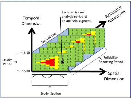
Source: Federal Highway Administration.
Required Inputs
The minimum required input data for the ATDM Analysis is:- Sufficient historic demand data and special event data to predict the variability of demand.
- Sufficient historic incident and weather data to predict the variability of capacity.
- Data required by selected traffic operations analysis tool.
Depending on the quality and detail of the available data more or less processing will be required to make it suitable for ATDM Analysis.
Acquisition and Processing of Demand Variability Data
Sufficient demand data must be gathered for the study period for the selected operations analysis tool, the HCM in this case. The HCM requires 15-minute demands throughout the study period. This might be a single day’s data, or it may be the average of several days. In addition, information on how study period demands will vary is required. The best source is archived count data for the facility (or facilities) to be studied. The data should be available for a sufficient number and cross-section of days for the analyst (and any stakeholders involved in the analysis) to be confident that nearly the true variability of demands for the study period has been captured.
Ideally, the analyst would have information on how each 15-minute period demand varied; however, information on how total study period demand varies is sufficient. The analyst then assumes that within peak period variations in demand were captured in the counts used to generate the demands for the traffic operations analysis tool. The between day variation for the entire peak period is then applied as a uniform factor applied to all the 15-minute demands within the peak. As a simplified example, assume the study period was one hour and 15-minute traffic volumes were recorded as 300, 400, 500, and 400 vehicles for total hourly demand of 1,600. Assume also that another scenario includes another day where the overall demand is 75% of the referenced (or seed day) indicated above. If similar 15-minute counts are not available, the methodology can used by applying a factor of 0.75 to each of the seed day 15-minute volumes resulting in assumed demand of 225, 300, 375, 300.
If sufficient archived demand data is not available, the analyst has two options: gather a sample of demands for the peak period over several days, or borrow archived data from a nearby permanent count station. The archived data for a nearby site is used to determine the day-to-day factors to be applied to a single day’s count data set for the facility to obtain an approximate estimate of the day-to-day variation in demands for the facility. The use of borrowed or default demand profiles will significantly affect the accuracy of the result. In any case, the demand profile is used as a basis for selecting the demand levels to be used in the overall analysis. For example, the analyst may determine that three levels of demand will be used: the 10th percentile demand, the mean demand, and the 90th percentile. Having the complete demand distribution makes identifying these levels straight forward.
Acquisition and Processing of Special Event Data
For most facilities, special events large enough and close enough to significantly affect facility operation are rare, and can therefore be ignored. Special events can be bundled into the overall demand variability data without requiring special consideration in the ATDM analysis.
For those facilities where major special events are a significant and frequent influence on facility operation then explicit consideration of special events may be warranted. This is especially true if the agency is evaluating ATDM investments specifically designed to address major events. Major league football, baseball, and basketball games, NASCAR races, state fairs, county fairs, and other events where attendance is expected to exceed 10,000 persons at any one time are examples of special events that may be worth evaluating for ATDM investments.
If special events are to be evaluated then the analyst will need to assemble vehicle arrival and departure peaking profiles and directions of travel for each of the events to be evaluated.
For each event the existing or proposed traffic control plan (cones, directional signs, stationing of traffic control officers, parking lot controls, etc.) will need to be defined by the analyst in sufficient detail for coding into the HCM analysis tool.
Acquisition and Processing of Weather Data
Hourly weather reports published by the National Oceanic and Atmospheric Administration (NOAA), Weather Underground, agency road weather information systems (RWIS), and other sources can be used to estimate the frequency of weather types for the facility. For the purposes of the reliability analysis the weather data must specify the historic frequencies of precipitation by type (rain, snow), the precipitation rate, the temperature and the visibility. Weather Underground’s historical hourly weather reports (which can be downloaded freely in .csv format from Weather Underground) contain all these metrics for almost every town and city in the United States.
The weather data must be classified into the appropriate HCM weather-type categories (light rain, heavy snow, etc.) which is different for freeways and urban streets. After classifying the weather observations, it is possible to compute the probabilities of weather occurrence for each weather type. In one year, there should be 8,760 (365*24) hourly observations. The probability of occurrence of a weather type is simply the ratio of the number of observations to 8,760. The annual hours per year of weather by type are used to compute the percentage frequencies (see Table 5).
When multiple weather types are present at the same time in the data, the analyst should classify the weather type as the one with the greatest effect on capacity (see capacity adjustment factors in Table 5 to identify which weather type has the greatest effect. The lower the factor the greater its effect on capacity.
Note: The minimum required weather data in this chart is the probability of occurrence during the reliability reporting period for each weather type. See Appendix A: Speed/Capacity for Weather, for the derivation of the capacity and speed adjustment factors shown here. Probabilities in this example chart are illustrative, not intended to represent actual conditions anywhere.
Acquisition and Processing of Incident Data
The ATDM Analysis method requires incident data for each of the specific incident type. Table 6 shows mean duration, effect on free-flow speeds, effect on capacity of the remaining open lanes, and the probability of occurrence within the study period (typically the weekday peak period) during the reliability reporting period (typically one year).
The analysis will be most accurate if archived incident data is available for the facility in the requisite detail. Lacking that, the required data can be estimated for existing conditions or forecasted for future conditions using Highway Safety Manual procedures, or the defaults described in Appendix B: Incident Probabilities and Duration. The effects of incidents on free-flow speeds and capacities of the remaining open lanes can be estimated using the defaults described in Appendix C: Speed/Capacity for Incidents.
Note: See Appendix B: Incident Probabilities and Duration, for the derivation of mean incident duration and probabilities. See Appendix C: Speed/Capacity for Incidents, for the derivation of the capacity and speed adjustment factors shown here. Probabilities in this example chart are illustrative, not intended to represent actual conditions anywhere.
Work Zone Data
If work zones are anticipated to be frequent and significant enough to affect annual traffic operations (or the ATDM investments to be tested are anticipated to significantly improve work zone traffic operations) then the analyst should identify the general frequencies of work zone by type, their duration, usual posted speed limits, and the number of lanes to remain open (see Table 7).
Note: The probabilities in this table are illustrative and are not based on a specific real-world location.
The probabilities are the proportion of study periods over the course of the reliability reporting period (typically a year) that are likely to have the designated work zone type and configuration present during the study period.
Work zones in place more than one day are generally classified as “long-term” work zones. On any given day, work zones may or may not be present and active during all or a portion of the daily study period. The duration entered in Table 7 is the number of minutes within the study period when the work zone is active. In this example, the work zone duration of 240 minutes indicates that the work zone is active for the entire 4-hour study period. Shorter work zone periods are certainly possible.
The work zone capacities per lane are shown in Table 7. They can be entered either in units of passenger cars per hour per lane, or vehicles per hour per lane, as long as consistent units are used for capacities throughout the table. The work zone capacity adjustment factors will then be calculated from that data. See Appendix D: Speed/Capacity for Work Zones for derivation of the capacity values and speed adjustments.
Data Required by Selected Operations Analysis Tool
The analyst must consult the users’ guide for the selected HCM operations analysis tool to determine what data is required for the tool. The general HCM input requirements for freeway analysis are given in Chapter 10 and subsequent chapters of Volume 2 of the 2010 HCM. For an arterial street analysis the HCM input requirements are given in Chapter 16 and subsequent chapters of Volume 3 of the 2010 HCM.
5.2 Step 2: Generate Scenarios
Overview
Highway capacity analyses are usually performed for near ideal conditions, clear weather, no incidents, recurring peak demand conditions. ATDM is designed to respond to non-ideal conditions. Thus, it is necessary to create scenarios of non-ideal conditions for evaluating the benefits of ATDM.
The ATDM Analysis methodology takes the approach of applying readily available and commonly used Highway Capacity Manual traffic operations analysis tools to static scenarios of demand, weather, and incident conditions rather than developing an entirely new tool. This approach gives the analyst more flexibility in the selection of operations analysis tools that are valid for the specific ATDM strategies under evaluation.
The computational and human resources required to generate inputs, compute performance, error-check, and evaluate results for each scenario set practical limits on the number of scenarios that can be considered for any given ATDM investment analysis. The objective of scenario generation is therefore to identify a sufficient number of varied representative scenarios to accurately evaluate the benefits of the specific ATDM investments that are under consideration without exceeding the resource constraints of the analyst. Because of these limitations, the ATDM Analysis methodology allows up to 30 scenarios to be considered.
As more sophisticated computational tools become available for generating and evaluating scenarios the resource constraints will become less of an issue for ATDM Analysis and numerous scenarios can be evaluated.
The ATDM Analysis method starts out by generating the full array of possible scenarios and then strategically selecting 30 scenarios for HCM analysis, thus enabling rapid analysis of the effects of ATDM strategies on facility performance.
The analysis framework allows for up to:
- 7 demand levels;
- 16 weather conditions;
- 13 incident conditions; and
- 7 work zone conditions.
The available demand, weather, incident, and work zone conditions combine to form 10,192 possible scenarios for analysis. Since it is not feasible with currently available HCM analysis tools for freeway analysis to evaluate this many scenarios the analyst must select 30 of these scenarios for analysis.
Note that the SHRP 2-L08 analysis tools enable the analyst to fully evaluate thousands of scenarios for reliability analysis. In the case of ATDM analysis, it is necessary to limit the number of scenarios to a much smaller number. The need to design and manually apply ATDM strategy responses for each scenario sets a practical limit on the number of scenarios that the analyst will want to create for an ATDM analysis.
The designation of demand, weather, incident, and work zone conditions, their combination into scenarios, and the selection of 30 scenarios for analysis are described in the following subsections.
Identify and Describe Demand Levels
The analyst identifies 7 possible levels of demand that may occur on the facility during the study period over the course of the many days included in the reliability reporting period.
The demand levels are developed from the historical or estimated historic demand data. The total study (peak) period demands for each day in the archive are ranked from lowest to highest. The 5th%, 15th%, 30th%, 50th%, 70th%, 85th%, 95th% highest values are then selected. If a complete (i.e., year-long) demand distribution is not available – either for the specific facility or for a similar one – the analyst needs to develop factors for determining key moments of the distribution that are applied to the short-count traffic data that are available. To do this, continuous volume data from an agency’s permanent count locations must be used. The process mirrors that used by traffic monitoring groups to develop daily and seasonal adjustments for daily short-duration counts to get an estimate of average annual daily traffic (AADT). The count locations are grouped by facility type and any other distinguishing factors (e.g., size of urban area). Then a complete distribution profile is developed. The factors assume that the data available to the analyst represent the mean values, so the factors are developed to predict various percentiles of the distribution as a function of the mean. For example, the analysis may show that the 80th percentile demand level is 1.1 times the mean.
Usually, the demand data needed for coding the traffic analysis tool is much more detailed than is available in the archives. Consequently it is usually necessary to collect the more detailed data for the tool for a single day (the seed day) and then factor those single demands to the target percentile demand level. The traffic analysis tool input seed day demands are compared to the target demand levels and factored up or down as necessary to match the target demand level. Unless the analyst has better data available, the same factor is applied to all input demands within the demand level.
The probability of each demand level is computed from the percentile values. The 5th percentile demand is assumed to be representative of the bottom 10% of demands. The 15th percentile demand is representative of demands between the 10th percentile and the 20th percentile, thus it has an estimated 10% probability, etc. (see Figure 8). In this example, the 5th, 15th, 30th, 50th, 70th, 85th, and 95th percentile demand levels are chosen.
Figure 8: Assignment of Probabilities to Percentile Demand Levels
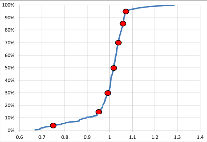
Source: Cambridge Systematics, Inc.
Table 8 shows an example outcome for this step. Seven demand levels have been selected from the demand profile for the facility. For each level a probability has been estimated along with an adjustment factor to be applied to the demands in the HCM seed file to create the demand level.
Note: The ratios shown here are illustrative. In this example the day that the analyst selected for counting the demands to be input into the HCM model happened to be about 2% above the average for the year.
In this example, special events have been subsumed within the demand levels selected for analysis. No separate special event demand levels are generated.
Define Weather Conditions
The ATDM Analysis method uses the freeway weather types identified in Chapter 10 (Freeway Facilities) of the 2010 Highway Capacity Manual. The available weather types are listed in Table 5. A total of 16 weather types are available for selection, including: clear weather and various intensities of: rain, snow, wind, temperature and visibility.
Each weather type for a scenario is assumed to apply to the entire study section of the facility for the entire study period.
Define Incident Conditions
The ATDM Analysis method uses the freeway incident types identified in Chapter 10 (Freeway Facilities) of the 2010 Highway Capacity Manual. The available incident types are listed in Table 6. A total of 13 incident types are available for selection, including: no incidents, noncrash incidents (breakdowns, debris), property damage only (PDO) crashes, injury crashes, and fatal crashes.
While incidents may occur randomly at any time and location within the study section and, study period, it is not feasible to evaluate all of these possibilities within 30 scenarios. Consequently, the analyst should select a representative location, start time, and duration for the incident. Since incidents are highly likely to cause congestion that spills over the temporal and geographic limits of the operations analysis tool, it is recommended that the analyst select an incident location near the downstream end of the study section and a start time near the start of the study period to more fully capture the incident effects.
Define Work Zone Conditions
The ATDM Analysis method uses the freeway work zone types identified in Chapter 10 (Freeway Facilities) of the 2010 Highway Capacity Manual. The available work zone types are listed in Table 7. A total of 7 types are available, including: no work zone; short-term work zones keeping 1, 2 or 3 lanes open; and long-term work zones keeping 1, 2, or 3 lanes open.
The ATDM Analysis method is indifferent to the name of the work zone type (long or short). The terms are included to enable the analyst to select different capacity and speed characteristics for long- and short-term work zones.
Work zones are treated as random events similar to incidents in the ATDM Analysis methodology.
While work zones can occur at any time and location within the study section, study period, and reliability reporting period, it is not feasible to evaluate all of these possibilities within 30 scenarios. Consequently, the analyst should select a representative location, start time, and duration for the work zones. Since work zones may cause congestion to spill over the temporal and geographic limits of the operations analysis tool, it is recommended that the analyst select a location near the downstream end of the study section and a start time near the start of the study period for the “representative” work zone to be included in the scenario analysis.
The duration of the work zone is set only for the time that the work zone persists during the study period. Work zone activity outside of the study period is not counted in the estimated duration.
Construction of Scenarios, Computation of Probabilities
The 7 demand levels, 16 weather types, 13 incident types, and 7 work zone types are combined into all possible combinations, resulting in 10,192 possible scenarios for analysis.
The analyst input the individual probabilities for each of the demand levels and types of weather, incidents, and work zones. These marginal probabilities are used to compute the combined probability of each scenario, assuming independence of the types and demand levels.
Equation 3
Where:
P(d,w,i,wz) = Combined probability of a scenario with demand level “d,” weather type “w,” incident type “I” and work zone type “wz.”
P(d) = Probability of demand level “d” (analyst input).
P(w) = Probability of weather of type “w” (analyst input).
P(i) = Probability of incident type “i” (analyst input).
P(wz) = Probability of work zone type “wz” (analyst input).
While it is not statistically correct to assume that demand, weather, incidents, and work zones are independent, as a first order approximation, the assumption of independence saves the analyst a greater amount of data collection to establish the correlations, and the resulting scenario probabilities give a rough indication of the relative frequency of one scenario compared to another.
The SHRP 2-L08 freeway method partially incorporated some limited correlation between demand and weather, and between weather and incidents by tying scenarios to specific months of the year. The natural correlation between season of the year, demand, weather, and incidents is incorporated into the monthly demand, weather, and incident rates used in the SHRP 2-L08 freeway method. The following equation illustrates this approach.
Equation 4
Where:
P(m, d,w,i,wz) = Combined probability of a scenario in month “m,” with demand level “d,” weather type “w,” incident type “I” and work zone type “wz.”
P(m,d) = Probability of demand level “d” during month “m” (analyst input).
P(m,w) = Probability of weather of type “w” during month “m” (analyst input).
P(m,i) = Probability of incident type “i” during month “m” (analyst input).
P(m,wz) = Probability of work zone type “wz” during month “m” (analyst input).
Selection of 30 Scenarios for HCM Analysis
At this point in the process, if all 7 demand levels, 16 weather types, 13 incident types, and 7 work zone types are considered, 10,192 possible scenarios for analysis will be generated. The analyst must then select 30 of those scenarios for analysis.
The need to reduce the analysis to 30 scenarios is not driven so much by computational requirements. Computer programs, properly written, can evaluate 10,192 scenarios in minutes if not seconds on today’s personal computers.
The need to reduce the analysis to 30 scenarios is driven more by the need of the analyst to fully specify the ATDM strategies to be employed individually for each scenario. At this point in time, given the early stage of ATDM development in the country, it is necessary to give the analyst complete freedom to specify the ATDM strategies for each and every scenario. Later, as the state of the art matures, it may be possible to write decision-making algorithms that will automatically select the appropriate ATDM strategies for each scenario. The ATDM Analysis method allows the analysts discretion, according to the analyst’s objectives for the ATDM analysis: The analyst selects 30 specific combinations of demand levels, weather, incidents, and work zones to be tested. This method guarantees that those combinations will be evaluated for the effects of ATDM. For example, if the analyst is evaluating the benefits of incident management investments, the analyst may wish to focus the scenario selection on those involving incidents. Table 9 illustrates one possible outcome using this method of scenario selection. When one attempts to use 30 scenarios to represent the effects for 10,192 scenarios, some detail must be sacrificed, and the danger of biasing the results in the selection must be recognized.
Note: Scenarios selected to achieve a target mix of conditions. d/c is the demand to capacity ratio.
5.3 Step 3: Apply Operations Model to Scenarios
In this step, the selected HCM operations analysis model is coded, error-checked, and calibrated, as appropriate. The analyst should consult the appropriate user’s guide for the selected tool.
The traffic operations analysis tool is applied separately to each scenario to compute predicted segment travel times for the facility under each scenario. For scenarios involving capacity reduction events such as weather, incidents, and work zones, the analyst will need to adjust the coded (or calibrated) capacities in the model to reflect those events.
Quality Control The Seed File
Often the demand inputs, traffic controls, and capacities reflect conditions measured in the field for a single day’s peak period (nonpeak periods could also be selected for analysis) (sometimes the analyst has sufficient data to average a few days of data into a “typical” peak period day. Either way, the result is a single representative study period coded into the traffic operations tool). The input file(s) for this initial operations model of the facility will be called the “Seed” file. The other scenarios are generated by pivoting off of this seed file. It is critical that this seed file be accurate as feasible, because the entire ATDM evaluation will based on this seed file.
5.4 Step 4: Compute MOEs (Before ATDM)
The MOEs (performance measures) reported by operations analysis tool for each scenario are combined to obtain the total performance statistics for the facility or facilities. Computation details are provided in Appendix E: Measures of Effectiveness.
The performance measures reported for the before condition are listed below:
- Vehicle-Miles Traveled Demand (VMT-Demand);
- Vehicle-Miles Traveled Served (VMT-Served);
- Vehicle-Hours Traveled (VHT);
- Vehicle-Hours Delay (VHD);
- System Efficiency: Average System Speed);
- Traveler Perspective: Vehicle-Hours Delay/Vehicle-Mile Traveled (VHD/VMT); and
- Reliability: the Planning Time Index (PTI) and the 80th Percentile Travel Time Index.
Table 10 shows a typical table of MOEs computed for a “Before” ATDM Analysis. From this table the summary statistics are computed with the results shown in Table 11.
The vehicle-miles demanded is the same as the amount traveled, indicating that all demand is served by the facility. The average speed for the study period over the days of the reliability reporting period is 58.1 mph (about 83% of the 70 mph free-flow speed for the facility. The average delay is 10.6 seconds per mile. The Planning Time Index (95th Percentile TTI) is 1.69. To be 95% confident of arriving on time over the course of a year of weekday PM peak periods, travelers must add an extra 69% to their expected free-flow travel time on the facility.
Note: VMT = vehicle-miles traveled. VHT = vehicle-hours traveled. VHD = vehicle-hours delay. TTI = Travel Time Index, W = Weather only, I = Incident Only, WI = Weather and Incident.
Note: Annual performance of facility during weekday PM peak periods before ATDM.
5.5 Step 5: Design ATDM Strategy
Overview
The current state of-the art for ATDM operations is rapidly evolving at this time. New strategies and the logic behind them are being developed, tested, and refined on a daily basis. This section describes a method for organizing the wide variety of possible ATDM system responses to changes in demand, weather, and incident conditions into a condensed menu of response plans, one for each situation suitable for a macroscopic analysis. The purpose of this analysis is to determine the potential operational and performance benefits of different general ATDM management approaches without requiring the analyst to evaluate and test every possible option and determine the precisely optimal decision rules, control settings, and tactics for each real life situation. Thus, this method is not suitable to determine the precise decision rules, control settings, and tactics that are optimal for a range of real life conditions. This method is designed to determine the likely benefits of introducing the control flexibility and responsiveness of ATDM to a facility.
This analysis method consequently condenses the wide variety of ATDM strategies into a simple menu of strategies that the analyst can select from to reflect different levels of investment and responsiveness of the ATDM strategies.
Appendix L: Designing an ATDM Program, provides an introductory overview of ATDM program design options and provides references for further information on ATDM program design.
The ATDM Analysis method currently provides for the analysis of the ATDM strategies listed in Table 12, along with a summary of how the method models each one.
As ATDM develops further more traffic management options will be available for both freeway and nonfreeway/arterial environment.
Travel Demand Management Strategies For Recurrent Congestion
Travel demand management (TDM) strategies can be everyday strategies designed to reduce recurrent congestion, or they may be incident, weather, and work zone-specific strategies designed to mitigate specific types of events on the facility. Those TDM strategies targeted to specific events will be dealt with as part of the response plans for those specific events. This section focuses on TDM strategies designed to address recurrent congestion.
Travel demand management options for recurring congestion included in the methodology are:
- Congestion pricing strategies, such as specific lane tolling or full facility tolling;
- Travel information strategies including pre-trip services such as web-based information and en-route information such as in-vehicle navigation devices, and changeable message signs; and
- Employer-based TDM strategies reflecting a wide range of employer incentives and disincentives to reduce single occupant vehicle commuting before the vehicle reaches the employer facility.
The various TDM strategies are bundled by the analyst into one or more TDM plans for the facility. The analyst then estimates the combined effects on demand of the strategies within each of the plans.
The analyst identifies the levels of demand when each TDM plan goes into effect. Each TDM plan is assumed to uniformly affect facility-wide demand for the entire study period for the scenario when the TDM plan is in effect.
The analyst may specify a different TDM plan, with a different effect on demand, for each of the 7 possible levels of demand identified by the analyst in the “before” analysis. Table 13 shows an example of TDM Plan coding.
Note: Entries are illustrative of a hypothetical TDM plan that becomes more aggressive (adding more TDM strategies) as demand increases, however; values shown are not intended to be representative of actual TDM effects. A value of 1.00 means no change with ATDM. Each row represents a different possible ATDM response for a different recurring demand condition.
Weather-Responsive Traffic Management Plan
Weather responsive traffic management (WRTM) plans consist of control strategies, traveler advisory strategies, and treatment strategies:
- Control strategies restrict the vehicles and imposes equipment requirements (such as chains) for vehicles using the facility during adverse weather;
- Traveler advisories include pre-trip and en-route information to advice drivers of weather conditions; and
- Treatment strategies include anti-icing and snow removal strategies among others.
The various weather traffic management strategies are bundled by the analyst into one or more WRTM plans for the facility. The analyst estimates the combined effects of the strategies within each plan on facility demand, capacity, and free-flow speeds. The analyst identifies the weather types when each WRTM plan goes into effect. Each WRTM plan is assumed to uniformly affect the entire facility for the entire study period when the weather type is present and the plan is in effect.
The analyst may specify a different W-TMP plan, with different effects on demand, capacity, and free-flow speeds, for each of the 16 possible weather types identified by the analyst in the “before” analysis. Table 14 shows an example of Weather TMP Plan coding.
Note: Entries are illustrative of the coding capabilities, not intended to represent actual Weather TMP effects. A value of 1.00 means no change with ATDM. Each row represents a different possible ATDM response for a different weather type. Weather dependent speed limits are coded by adjusting the free-flow speed for each weather type.
Traffic Incident Management Plan
The Traffic incident management (TIM plan) consists of site management and control strategies, traveler advisory strategies, plus detection, verification, response and clearance strategies.
- Site management and traffic control include strategies such as: incident command systems (on-site traffic management teams and end of queue advance warning systems); travel information strategies (including pre-trip services such as web-based information and en-route information such as in-vehicle navigation devices, and changeable message signs); detection and verification strategies (including field verification by on-site responders, closed circuit television cameras, enhanced roadway reference markers, enhanced/automated 911 positioning systems, motorist aid call boxes, and automated collision notification systems);
- Response strategies such as: personnel/equipment resource lists; towing and recovery vehicle identification guides; instant tow dispatch procedures; towing and recovery zone-based contracts; enhanced computer aided dispatch; dual/optimized dispatch procedures; motorcycle patrols; and equipment staging areas/prepositioned equipment; and
- Quick clearance and recovery strategies such as: incident investigation sites; quick clearance laws, policies, and incentives; expedited crash investigations, service patrols, enhanced capability service patrols; and major incident response teams.
The various traffic incident management strategies are bundled by the analyst into one or more TIM plans for the facility. The analyst estimates the combined effects of the strategies within each plan on facility demand, capacity, and free-flow speeds. The analyst identifies the incident types when each TIM plan goes into effect.
Each TIM plan is assumed to uniformly affect demand for the entire facility for the analysis time periods when the incident is present and the TIM plan is in effect. Capacity and free-flow speeds are assumed to be affected by the TIM plan only in the vicinity of the incident, while it is present. Variable speed limits (see next section) are assumed to be in effect (if active) only upstream of the incident and only while the incident is present.
The analyst may specify a different TIM plan, with different effects on demand, capacity, incident duration, and free-flow speeds, for each of the 13 possible incident types identified by the analyst in the “before” analysis (see Table 15). Alternatively, the analyst may apply a particular TIM plan for more than one incident type.
Note: Entries are illustrative of the coding capabilities, not intended to represent actual TIM effects. A value of 1.00 means no change with ATDM. Each row represents a different possible ATDM response for a different incident type. VSL = variable speed limit.
Variable Speed Limits (VSL) or Speed Advisories
Variable speed limits may be applied four ways in the analysis methodology.
- The analyst may specify uniform (constant) reductions in the facility free-flow speed for each of the 7 available demand levels.
- The analyst may specify uniform (constant) reductions in the facility free-flow speed for each of the 16 possible weather types.
- The analyst may specify reduced free-flow speed in the vicinity of an incident and specify the graduated reduction in upstream free-flow speeds as traffic approaches the incident, while the incident is active.
- The analyst may specify reduced free-flow speed in the vicinity of a work zone and specify the graduated reduction in upstream free-flow speeds as traffic approaches the work zone, while the work zone is active.
For VSL when traffic incidents or work zones are present, it is assumed to apply only upstream of the incident or work zone, and only while the incident or work zone is active. The analyst must translate the reduction in speed limit into the equivalent reduction in free-flow speed. For speed advisories, it is assumed that motorists comply with the recommended speed; there is no provision in the methodology to adjust for compliance rate. If the analyst believes this assumption to be untenable, then speed advisories should be selected as a strategy.
Note that the input VSL speed for a segment will be overridden if it violates the HCM 2010 requirement that the free-flow speed be higher than the speed at capacity (which is estimated by the HCM 2010 assuming a density of 45 passenger car equivalents per lane per mile).
Work Zone Traffic Management Plan
The work zone traffic management plan (WZ-TMP) consists of site management and control strategies, and traveler advisory strategies. Site management and control strategies include end of queue advance warning signs, speed feedback signs, and automated speed enforcement, in addition to the conventional work zone traffic management strategies. Travel information strategies including pre-trip services such as web-based information and en-route information such as in-vehicle navigation devices, and changeable message signs.
The various work zone traffic management strategies are bundled by the analyst into one or more WZ-TMP plans for the facility. The analyst estimates the combined effects of the strategies within each plan on facility demand, capacity, and free-flow speeds. The analyst identifies the work zone types when each WZ-TMP plan goes into effect.
Each WZ-TMP plan is assumed to uniformly affect demand for the entire facility for the analysis time periods when the work zone is present and the WZ-TMP plan is in effect. Capacity and free-flow speeds are assumed to be affected by the WZ-TMP plan only in the vicinity of the work zone, while it is present. Work zone triggered variable speed limits (see previous section) are assumed to be in effect (if active) only upstream of the work zone and only while the work zone is present.
The analyst may specify a different WZ-TMP plan, with different effects on demand, capacity, and free-flow speeds, for each of the 7 possible work zone types identified by the analyst in the “before” analysis.
Note: Entries are illustrative of the coding capabilities, not intended to represent actual Work Zone TMP effects. A value of 1.00 means no change with ATDM. Each row represents a different possible set of ATDM strategies for a different work zone type. VSL = variable speed limit.
HOV/HOT Lane Management Strategies
The ATDM Analysis methodology is set up to evaluate 5 possible HOV and HOT (Express) lane management strategies in response to demand, weather, incidents, and work zones.
- No change to “before” conditions.
- Convert one or more mixed-flow lanes (coded in the seed file) to HOV lane(s).
- This option is provided in the methodology to overcome the lack of an HOV lane analysis capability in the HCM 2010 freeway analysis procedure.
- This option reduces the capacity of the mixed-flow lane(s) to the user specified value for the HOV lane(s). This value is compared to the user specified number of HOVs likely to use the HOV lane(s) and the lower of the two values is the selected capacity for the HOV lane(s). A weighted average capacity across all lanes is then computed to obtain the final capacity adjustment factor used in the scenario. It is assumed that the number of carpools using the HOV lane is exactly the value specified by the user. The HCM 2010 does not provide a procedure to estimate the performance of only the HOV lane. The methodology uses the lower HOV lane capacity to estimate the average capacity across all lanes on the freeway. This accounts for the fact that the mixed-flow lanes may be more congested than the HOV lane, because SOVs are not allowed to use the HOV lane, and some eligible HOVs choose to not use the HOV lane (for various reasons, including needing to exit at the next off-ramp) (the average freeway speed computed using the HCM curves and the method’s average capacity probably underestimates the speeds in the HOV lane).
- Open the HOV lane(s) up to all traffic. The HOV lane becomes a mixed-flow lane with the capacities and free-flow speeds typical of the other mixed-flow lanes in the segment.
- Convert one or more mixed-flow lanes (coded in the seed file) to HOT lane(s) with the capacity per lane identified by the user.
- This option assumes that the toll will be dynamically set as low as necessary to equalize demand across all lanes until the HOT lane(s) capacity is reached, at which point the HOT lane(s) capacity will control.
- Open the HOT lane(s) up to all traffic with no toll. The HOT lane(s) become in essence mixed-flow lane(s) with the capacities and free-flow speeds typical of the other mixed-flow lanes in the segment.
Due to limitations of the HCM 2010 freeway analysis procedure, all HOV and HOT lanes must extend the full length of the freeway and must be continuously accessible from the mixed-flow lanes (no barrier separation).
The analytical details for these options are given in Appendix G: Speed/Capacity for HOV/HOT Lane Strategies.
Shoulder and Median Lane Strategies
Seven strategies for temporary use of shoulder and median lanes are available in the ATDM analysis framework (in addition to the “no change” option).
- No change to “before” conditions.
- Shoulder lane temporarily opened up as an auxiliary lane between the on-ramps of the facility and the off-ramps.
- The shoulder lane is opened continuously over the length of the facility to buses only.
- The shoulder lane is opened continuously over the length of the facility to HOVs only.
- The shoulder lane is opened continuously over the length of the facility to all vehicles.
For median lanes, the same options are available as for shoulders, with the exception that median auxiliary lanes is not available as an option. More analytical details on capacities and speeds for these options are provided in Appendix H: Speed/Capacity for Shoulder/Median Lane Strategies.
Truck Controls
Two options are available for truck controls: “Base” (no change from the seed file), or “Truck Ban,” which removes the user specified number of trucks (specified by the user as a percentage of the total traffic stream).
The user-specified PCE value per truck is used along with the percent trucks to compute the capacity adjustment factor for the freeway.
The user specified percent of trucks is used to compute the demand reduction factor (1% trucks) to be applied to all facility demands.
The user should verify that his or her entries for percent trucks and PCEs are consistent with the user’s entries in the seed file for percent trucks and general terrain type. Since it is possible for a gross vehicle weight limit to affect less than 100% of the trucks on the freeway with 6 tires, the percent trucks entered by the user for the truck ban can be less than or equal to the total percent trucks on the facility.
A truck ban is assumed to apply to the full length of the freeway for the entire duration of the study period.
Until such time as the HCM 2010 freeway method has a procedure for estimating the effects of trucks on average free-flow speeds, the ATDM analysis procedure assumes that a truck ban would have no effect on facility free-flow speeds.
Ramp Metering
Three ramp meter strategies are provided in the ATDM Analysis methodology, in addition to the “no change” option.
- No change to “before” conditions.
- Meters operating at fixed (potentially varying by time of day) rates during the study period.
- Meters operating in dynamic local optimal mode. Each ramp meter optimizes its own rate based on the freeway mainline volumes immediately upstream and downstream of the ramp.
- The methodology sets the meter rate for each 15-minute analysis period at each ramp as the difference between the target mainline maximum downstream freeway flow rate and the upstream mainline freeway flow rate for the segment where the ramp is located (subject to the user specified maximum and minimum rates per on-ramp lane).
Additional analytical details are provided in Appendix I: Speed/Capacity for Ramp Metering Strategies.
5.6 Step 6: Convert Strategy into Operations Inputs
In this step the ATDM response plans specified in the previous step are converted into the appropriate traffic operations analysis input parameters.
For scenarios where multiple plans are in effect (for example, an incident in a work zone during bad weather), then (with the exception of the free-flow speed adjustment factor) the effects are multiplied together (assuming independent multiplicative effects). The individual demand or capacity effects for each plan are multiplied to obtain the combined effect of multiple ATDM plan responses.
The exception to this assumption is the free-flow speed adjustment factor. The combined effect is assumed to be the minimum of each of the plan factors. Thus for an incident (with a normal speed adjustment of 0.50) occurring in a work zone (with the work zone speed adjustment being 0.75), the combined effect on free-flow speed is assumed to be the minimum of the two plans, or 0.50, not the two factors multiplied together.
5.7 Step 7: Apply Operations Analysis Tool (“After” Analysis)
This step involves coding the ATDM strategies into each of the operations analysis model input files for the demand/capacity scenarios. For some ATDM strategies, such as time-of-day ramp metering, a single set of adjustments may apply to all of the demand and capacity scenarios. For traffic responsive and incident responsive ATDM strategies the adjustments may vary not only by scenario but also for each time slice within the scenario. The analyst may find it desirable to create a “control emulator” that reads the demands each time slice within each demand and capacity scenario and applies the appropriate capacity and control adjustment, to automate the adjustments. Table 17 shows how this process may be automated for each ATDM strategy.
Note: a If user does not agree with automated application approach shown in table, user can post-process the recommended adjustments by analysis period and segment.
b User Specified: User must specify scenario to which the control strategy applies.
In cases where the ATDM measure is expected to influence the frequency, severity, or duration of incidents, then the probabilities of the capacity scenarios with incidents will need to be modified as well. A full discussion on developing both “before” and “after” incident probabilities follows. Reductions in incident duration times are dependent on the type of traffic incident management strategy deployed.
Estimating “Before” Probabilities for Incidents
Ideally, the analyst has access to complete incident data logs for a metropolitan area or an extended facility from which the probabilities for each incident level in the experimental design can be developed directly. If this is not possible, a simple method for estimating the probabilities associated with various incident categories pivots off of information on crashes, which are a subset of total incidents. Roughly 15-30% of total incidents are crashes; for the purpose of this report, a value of 20.4% is used, based on data from the SHRP 2-L08 research. Wherever possible incident data logs should be used to develop local values for this factor. The expected number of annual incidents on facility for a particular time period is then:
E(inc) = PeriodVMT x CrashRate x IncidentProportionFactor
The incident proportion factor is the reciprocal of the percent of total incidents that are crashes. Using the default value from SHRP 2-L08, this is 1/0.204 or 4.9. Note that the VMT is computed for the entire year must apply only for the period being studied, e.g., weekday/nonholiday peak period.
If the analyst wishes, the Highway Safety Manual can be used to estimate the expected number of annual crashes, which are then factored up to annual incidents using the Incident Proportion Factor.
Once the expected number of annual incidents is obtained, it is assumed that no more than one occurs each “day” on the facility. In reality, more than one can occur on a day, but the analytic method is not capable of modeling this situation. However, the total number of annual incidents is preserved by assuming that the number of days with incidents in a year is equal to the total annual incidents. The probability that any kind of incident occurs on the facility over the course of a year is then the expected number of incidents divided by the number of days in a year represented by the analysis period. For example, consider that we have estimated that 90 incidents occur during the AM peak period for weekday/nonholidays. This represents 90/250 = 36%. So, the probability of having an incident–free day is 64%.
The next step is to break out the 36% total incident probability into the levels chosen by the analyst. This is done by using the incident distributions presented earlier, maintaining the relative proportions between categories.
Impacts of Strategies Affecting Incident Frequency (Occurrence)
Several ATDM strategies – as well as traditional safety countermeasures – reduce the frequency of crashes on facilities. A simple method for accounting for the positive effect of some strategies on crashes adjusts the probabilities previously defined for the incident factor in the experimental design. The following example will illustrate the method.
The analyst has already defined the following levels and probabilities for the incident dimension:
- No incident: 70%;
- 1 lane blocked, 30 minutes: 20%; and
- 2+ lanes blocked, 30 minutes: 10%.
In the above distribution, the probability of an incident is 30%. If the analyst is considering weekday/nonholidays (250 days per year), then the expected number of total incidents is: 0.30*250 = 75. Implementing a safety improvement on the facility is expected to reduce crashes by 18%, based on published crash reduction factors. Assuming that crashes are 20.4% of total incidents, the expected reduction factor for total incidents is: 0.18*0.204 = 0.037. Total incidents are then calculated to be: 75*(1 – 0.037) = 72.2, or 28.9% of weekday/nonholidays. Therefore, the number of days with no incident is: 1 – 0.289 = 0.711. To complete the example, we keep the proportions for the incident categories constant, in this case, 2:1.
- No incident: 71.1%;
- 1 lane blocked, 30 minutes: 19.3%; and
- 2+ lanes blocked, 30 minutes: 9.6%.
5.8 Step 8: Compute MOEs (“After” Condition)
The “After” MOEs are computed for each demand/capacity scenario using the same procedures as were used for the “before” case.
Adjustments for Congestion Spill Over
In cases where the estimated queues spill over the temporal and/or spatial limits of the operations analysis tool then the best solution is to expand the limits of the tool and rerun the analysis. The limits should be revised if the spillover is frequent, occurring in many scenarios with cumulative probability of greater than 10%.
However, if the cumulative probability of those scenarios with spillovers is less than 10%, then the analyst may consider whether resource constraints, the low probabilities of such extreme scenarios, and cost-effectiveness considerations, may limit the ability to expand the limits. In such situations, it is necessary for the analyst to work with the study stakeholders to:
- Assess the probability (and therefore the significance) of the scenarios causing the overflow;
- Assess the degree to which not accurately modeling the overflows will introduce bias that would significantly affect the decisions regarding ATDM investments, and, if significant;
- Determine if a reasonable increase in the study limits will adequately capture the overflows, and if not;
- Approximately account for the congestion spill over outside of the operations analysis tool limits. Use the methodology described in Step 4.