Measuring Border Delay and Crossing Times at the U.S.–Mexico Border—Part II
Guidebook for Analysis and Dissemination of Border Crossing Time and Wait Time Data
Final Report
DATA ANALYSIS
Key Steps for Analyzing the Data
Analysis of RFID-based border crossing time and wait time measurement system data, both real-time and archived, revolves around two main objectives: (1) creating advanced traveler information, and (2) developing performance measures about an individual border crossing. For both purposes, data analysis starts with processing raw data, which is defined for the purposes of this guidebook as segment travel time, crossing time, or wait time of an individual truck (detected through its RFID transponder) based on its re-identification by the RFID readers at different locations of the border crossing.
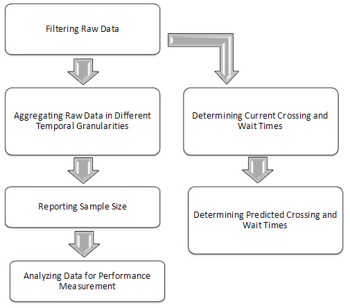
Processing the raw data needs to include a filtering process to eliminate erroneous and duplicate data prior to converting real-time data into either traveler information or performance measures (if real-time data are correct, then archived data are also). Once a filtered collection of raw data is obtained, it then needs to be aggregated into different temporal granularities, which then are used to create traveler information and performance measures. It is recommended that visibility and traceability of the raw data processing be maintained for quality assurance and to validate data analysis results.
Key steps for analyzing the data, including processing raw data, aggregating the processed data, and determining performance measures, are illustrated in Figure 2.
The data analysis approach utilizes four key dimensions of congestion—duration, extent, intensity, and reliability—to characterize performance of freight movements at a border crossing.[2] Duration is the length of time during which congestion at the border affects the freight movement. It is measured by determining the number of hours the facility operates below acceptable conditions, such as off-peak or optimal speed/travel time. Extent is described by estimating the number of vehicle/trips affected by congestion. This can be measured by determining the number of trips that experience crossing time or wait time above an acceptable condition or an established baseline. Intensity is the severity of congestion and is measured by average travel time and delay. Reliability measure variation in the amount of congestion for buffer time and buffer index is used.
This project’s final report includes detailed information about the tools (i.e., hardware, software, and tables) used for data analysis for the BOTA POE. Table 1 gives examples of the archived and aggregated data used at the BOTA and Pharr POEs.
| Table Name | Description |
|---|---|
| Raw Crossing Time | Stores crossing time of individual commercial vehicles. |
| Average Crossing Time, 15 and 60 Minutes | Stores average crossing time of northbound commercial vehicles calculated every 15 and 60 minutes. |
| Raw Wait Time | Stores wait time of individual commercial vehicles. |
| Average Wait Time, 15 and 60 Minutes | Stores average wait time of northbound commercial vehicles calculated every 15 and 60 minutes. |
| 15- and 60-Minute Tag Count | Stores, in 15- and 60-minute intervals, total count of transponders identified by individual RFID readers. |
| Monthly Performance (Dashboard) | Stores monthly performance indicators for northbound commercial vehicles at POEs. Indicators include average crossing and wait time, buffer index,2 95th percentile,3 and incoming volume. |
| Daily and Monthly Total Crossing Time Delay | Stores total crossing delay calculated at daily and monthly intervals based on average and 95th-percentile values as optimal crossing time. |
| Daily and Monthly Total Wait Time Delay | Stores total wait delay of commercial vehicles calculated at daily and monthly intervals based on average and 95th-percentile values as optimal crossing time. |
| Daily and Monthly Average Delay per Truck | Stores daily and monthly average delay of commercial vehicles calculated based on average and 95th-percentile values as optimal crossing time. It includes two separate fields to reflect wait time as well as crossing time delay. |
| Daily and Monthly Percentage of Trucks Congested | Stores daily and monthly percentage of trucks congested, which is calculated based on average and 95th-percentile values as optimal crossing time. It includes two separate fields to reflect wait time as well as crossing time delay. |
| Monthly Incoming Freight Volume | Stores monthly total freight containers entering the United States by various modes of transportation and container type (empty and loaded). |
| Monthly Import-Export Volume by Mode | Stores monthly total trade value and weight with origin as Mexico and destination States in the United States by mode of transportation. |
| Monthly Import-Export Volume by Commodity | Stores monthly total trade value and weight with Mexico by commodity. |
| Monthly Incoming Vehicle Volume | Stores monthly total vehicles entering the United States by various modes of transportation through various border regions in the State of Texas. |
Subsequent sections describe additional details about the data analysis approach.
Processing Raw Data
The RFID-based border crossing time and wait time measurement stations in the field send identification and time stamps of individual transponders from the remote stations to a central server, and the data are stored in database servers in a relational database structure. For the purposes of this guidebook, raw data represent crossing times, wait times, and segment travel times of individual trucks (i.e., transponders). As the transponder information arrives in the central server, individual crossing and wait times are calculated after identification of transponders are matched by subsequent RFID readers. Raw data are then stored in a table, which is constantly updated using a trigger mechanism in the database as new transponders are re-identified. The RFID-based border crossing time and wait time measurement system is involved in more than just data collection. It also plays a role in data analysis and dissemination.
Filtering Raw Data
Depending on the characteristics of border crossings, a significant number of trucks could be part of drayage or other operations that result in their crossing the border several times in a day. Hence, it is imperative that a process to filter raw data be able to distinguish individual one-way trips inbound to the United States. This can be achieved by using a fixed time window. This is the minimum value a truck needs before the truck can join the queue again for making subsequent trips across the border. For example, if this time window is 120 minutes, it is assumed that a truck typically takes more than that amount before returning to join the queue to cross the border again. However, this value needs to be reflective of the crossing time at the POE and thus needs to be much higher than crossing time of trucks even if some of them go through secondary inspection. It should be noted that the current filtering technique most likely filters out secondary inspection. Also, the value must not be so high that it is possible that trucks can cross the border again within that time period.
Table 2 illustrates some examples of how the fixed time window filtering set at 120 minutes might work.
| Vehicle Transponder ID | Measured Crossing Time | Data Acceptance |
|---|---|---|
| Transponder A | 45 minutes | Yes |
| Transponder B | 110 minutes | Yes |
| Transponder C | 135 minutes | No |
In some cases, transponders can be read more than once by the RFID readers at the same instance (or within a span of a few seconds), resulting in multiple records of raw data. The reason why RFID readers do that is unknown; however, such duplicate records need to be removed from the database using built-in query functions.
Aggregating Raw Data
Depending on the performance measures to be calculated, raw data need to be aggregated into different temporal granularities. Average crossing and wait times from the raw data can be determined using the following techniques:
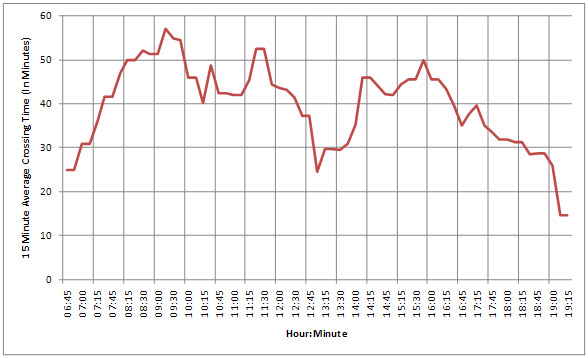
- Determine average crossing and wait times at a predefined frequency (e.g., every 15 minutes). For example, determine average crossing and wait times at 7:00 AM, 7:15 AM, and so on. This technique requires using a block of raw data, the span of which could be a fixed time window (e.g., 120 minutes), to calculate the average crossing and wait times. In addition to average values, standard deviation can also be part of the calculation. Average values reported every 15 minutes can be used to monitor trends within a day or week or within a predefined time period. They can also be used to identify peak and off-peak periods. Figure 3 shows 15-minute average crossing time measured at BOTA.
- Aggregate travel time by averaging the raw data for an entire day, week, and month. This technique is useful in monitoring long-term trends of border crossing performance but dampens the peaks and off-peak values of crossing and wait times.
Reporting Sample Size
For the purpose of this guidebook, a sample is referred to as a filtered set of crossing or wait time values of one or more trucks. When aggregating crossing and wait time values, it is a good practice to also report the sample size used in the calculation. This demonstrates the representativeness of the calculation.
Sample size for individual reporting periods, such as hourly, daily, weekly, and monthly, also assists in understanding the performance of the RFID system as well as the underlying trend of truck volume crossing the border.
One of the questions stakeholders frequently ask is, “What is the minimum sample size needed to aggregate border crossing and wait times to remain statistically significant?” While that number has not been established scientifically for trucks passing RFID reader stations at POEs, a minimum sample size can be approximated by using a mathematical technique known as the coefficient of variation (CV).
It is common knowledge that sample size is a function of variability in the data, also measured by the CV, which is a ratio of standard deviation of the sample and the mean. The higher the CV, the more samples required to represent the population. Using the following relationship (t-statistics), a quick analysis of minimum sample size required in a day can be determined by using the following equations:
![]()
![]()
![]()
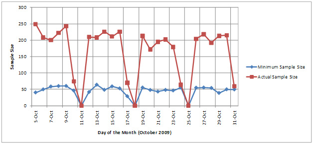
While these equations are widely used, an implementing agency needs to verify their appropriateness for the agency’s purpose. Figure 4 shows daily minimum sample size, estimated using the coefficient of variation, and actual sample size (for crossing times) obtained from the RFID-based border crossing time and wait time measurement system deployed at BOTA in October 2009. The actual sample size was well above the minimum sample size. However, two key concepts need to be recognized:
- If the system allows, minimum sample size needs to be separately estimated for individual types of shipments (e.g., FAST, non-FAST) because the coefficient of variation most likely is smaller for individual types of shipments than when combining the crossing times or wait times for all shipment types.
- Sample size required to relay traveler information within an hour of the timeframe is not the same as calculating daily performance measure.
During the writing of this guidebook, the RFID-based border crossing time and wait time measurement systems deployed at BOTA and Pharr cannot separate crossing times and wait times for individual shipment types since non-FAST shipments are known to use lanes to FAST Primary Inspection booths.
Analyzing Data for Traveler Information Purposes
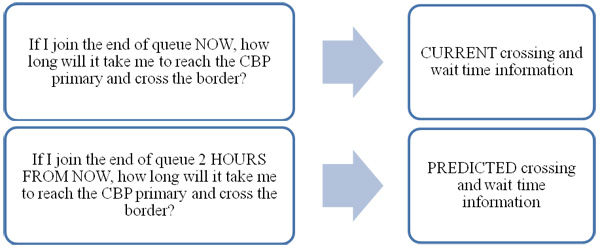
The main goal of providing traveler information to stakeholders (e.g., freight carriers, dispatchers) is to be able to let the stakeholders know current and future conditions at border crossings. The RFID-based border crossing time and wait time measurement system has the capability to inform the stakeholders about current and predicted values of crossing and wait times and to indicate extreme events such as unplanned closure of a border crossing. Also, crossing and wait time information can be integrated with number of lanes open and closed to give the stakeholders a sense of what is to be expected at the border in terms of long or short crossing and wait times. Figure 5 shows questions for which freight carriers and dispatchers seek answers from current and predicted crossing and wait times. Certainly, it is technically feasible to refine the questions to seek current and predicted crossing and wait times for the type of load freight carriers are to be moving (e.g., empty, non-FAST, FAST).
Determining Current Crossing and Wait Times
Current crossing and wait time information provides freight carriers advanced information on the current condition at the border crossing. A simple algorithm to average the most recent block of raw data is sufficient to estimate current crossing and wait times. At a predefined interval (or update frequency), the algorithm finds a block of filtered raw data and calculates the average crossing or wait times of trucks using a predefined time window. Another method is to find the block of transponders that were read between the start and end time and then filter the crossing or wait time data and calculate a simple average. At BOTA, the current crossing time is determined using the following procedure:
- Average crossing times are calculated every 15 minutes (e.g., 9:00 AM, 9:15 AM, 9:30 AM.).
- The procedure uses 120 minutes as the time window, meaning this value is used as a maximum crossing time.
- To calculate average crossing time at 9:00 AM, all the transponders that were read between 7:00 AM and 9:00 AM are matched and travel times of matched tags are averaged.
Unfortunately, there are no standard procedures based on which update frequency can be established. It is up to the discretion of the implementing agency to establish frequency at which to update the information. However, it needs to be consistent with updating frequency that can be achieved by field display devices (e.g., dynamic message signs [DMSs]). While DMS updates are typically made by operators and thus limited in update frequency, Web sites and Real Simple Syndication (RSS) feeds do not have limitations as to how frequently information can be updated. Agencies also use different update frequencies depending on peak and congested condition versus off-peak conditions, e.g., higher frequency during peak and congested conditions and lower frequency otherwise. This is because travelers and freight carriers tend to be more anxious for information during peak and congested conditions.
Determining Predicted Crossing and Wait Times
Predicting crossing and wait times of trucks crossing the border is challenging in terms of finding efficient analysis techniques. Implementing agencies need to be cognizant that developing such a prediction model might constitute a separate project or a major task by itself. Hence, the implementing agency needs to confer with stakeholders on identifying benefits of providing predicted crossing and wait times at the border. Some of the key questions that need to be answered before attempts are made to develop prediction algorithms are the following:
- What is the appropriate prediction horizon? Accuracy and reliability of prediction algorithms decrease as prediction horizon increases. The implementing agency needs to consult with the affected freight shippers and dispatchers to determine appropriate prediction horizon.
- What is the impact of variability of data? Very high variability in raw data results in unreliable and less-than-accurate prediction values. Also, it is difficult to define thresholds for high and low variability that produce reasonably accurate predicted crossing and wait times. However, variability can be reduced if the RFID-based border crossing time and wait time measurement system can distinguish crossing and wait times for different types of truck loads.
- What is the perception of accuracy among stakeholders? Perception of accuracy of the predicted crossing and wait times after the fact vary depending on individual carriers unless the prediction algorithm is sensitive to external factors such as type of shipment being transported, time of day, and day of week. Hence, over time, motor carriers may complain about accuracy and reliability of the predicted values.
The majority of prediction models use historical (archived) data with an assumption that day-to-day trends remain similar over a short period of time (e.g., weeks instead of years). Time-series models rely on historic trends and do not use input/output or parametric estimation to predict future values. They are easier to compute and easier to implement but are not sensitive to sudden changes in operational conditions at the border. Prediction models based on queuing theory may not be efficient because of highly random (and often unknown) inspection times.
Analyzing Data for Performance Measurement
From a planning and long-range performance monitoring perspective, archived data can be used to determine four key dimensions of congestion—duration, extent, intensity, and reliability. The following performance measures are recommended to measure those four dimensions of congestion:
- Summary statistics on raw crossing and wait time data.
- Average crossing and wait times.
- Buffer time and buffer index.
- Delay.
- Length of peak periods.
- Percentage of total trips that were congested.
Implementing agencies can then present the above measures in different temporal granularities for use in various transportation applications (see Obtaining Stakeholder Input for Data Analysis and Dissemination section for examples).
Summary Statistics about Raw Data
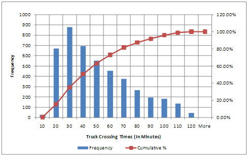
Summary statistics of raw crossing and wait time data include histograms of raw data collected on a typical day/week/month. Summary statistics provide two very important observations on the conditions of freight movement across the border—average (and other percentile) crossing and wait times and variability of crossing and wait times at the border. By having quantified values of crossing and wait times, there is no need to depend on anecdotal values of actual crossing and wait times at the border. Reliability of crossing and wait times can be a powerful tool for trade groups and other stakeholders concerned with transportation improvements to be made at the border. Figure 6 shows histograms of crossing times obtained from the RFID system deployed at BOTA. The histograms show that 95 percent of trucks take approximately 100 minutes or less to cross the border, and 50 percent of trucks require approximately 40 minutes or less to cross the border.
Aggregating Raw Crossing and Wait Time Data
Raw crossing and wait time data can be aggregated by calculating averages of blocks of raw data at predefined time intervals using the following procedure.
For example, to calculate average travel time between entry and exit reader stations at 9:00 AM, all the tags that were read between 7:00 AM and 9:00 AM are matched and travel times of matched tags are averaged (simple mean). The entry reader station is located at the end of the queue of trucks inbound to the United States, and the exit reader station is located where the trucks exit on the U.S. roadway system after all inspections. The average travel time is calculated every 15 minutes (e.g., 9:00 AM, 9:15 AM, 9:30 AM). The procedure uses 120 minutes as the time window, meaning this value is used as a maximum travel time that could occur at any given segment and total crossing time. However, the length of the time window is unique to each border crossing and is adjustable.
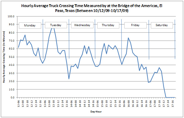
Figure 7 shows daily variation of hourly average crossing times at BOTA for an entire week.
It is important to understand the nature of the data collected in order to be able to factor in trends needed to support proper analysis. For example, average crossing and wait times determined by taking the average of an entire month or week of data may downplay the peak and off-peak values of crossing and wait times. Differences in monthly averages of crossing times and wait times from one year to the next may be subtle and insignificant unless a major improvement or event occurred between those years. However, it is entirely possible that when viewing monthly averages over a longer period (e.g., several years), the data might show a definitive trend. One way to ensure the peaks and valleys are reflected in the analyses is to compare small blocks of data (e.g., same week of year, same month of year).
Determining Buffer Time and Indices
For freight carriers, significant variation in travel time can impact inventory planning and the efficient use of transportation infrastructure, particularly for time-sensitive goods due to value, perishability, or business operating characteristics (such as just-in-time delivery operations). Specifically, delays in crossing the border are likely to have significant adverse economic effects. Longer travel times are an important issue, but the assembly process can be adjusted to accommodate them; it is more difficult to accommodate unpredictable crossing and wait times. However, freight shippers and manufacturers are also concerned about travel time variability (the variation in travel time) and reliability (which relates to reaching destinations at expected times) because those factors are beyond their capability to influence.
Two performance measures that gauge variability and reliability are buffer time and buffer index.
Buffer time is a measure of travel (any percentile could be used) and the average time for all trucks—it represents the extra time a driver must budget to cross the border at the average time with a 95 percent certainty. This percentage is used for illustration purposes and can be varied based on user expectations, e.g., 75 percent or 50 percent. Increasing buffer times reduces the possibility that the driver arrives late for an appointment. Buffer time can also be reported for time of day, day of week, month, and so forth.
Buffer index is the extra time that is required to cross the border than usual (average) and indicates reliability of the service. Buffer index expresses the amount of extra buffer time needed to be on time for 95 percent of the trips (e.g., a late shipment on one day per month). (Again, 95 percent is used for illustration and can be varied based on user expectations.)
Buffer index can also be reported for time of day, day of week, month, and so forth. This is the measure that is most comparable on an annual basis and between crossings, as it standardizes the measure by removing variables such as crossing length.
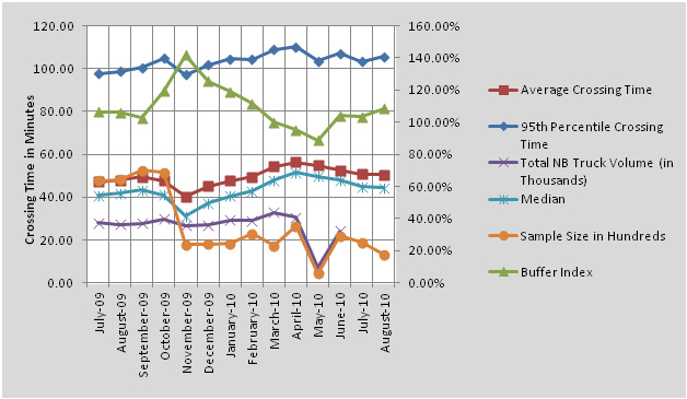
Figure 8 shows monthly variation of buffer index coupled with volume and 95th-percentile crossing time for BOTA. The left vertical axis represents indices related to crossing time (average, 95th percentile, and median) in minutes and the truck volume in thousands, which was provided by CBP. The right axis represents buffer index, which measures the reliability of travel service and is calculated as the ratio between the difference of the 95th-percentile crossing time and the average crossing time divided by the average crossing time.
Determining Delay Measures
For the purposes of this document, border delay is defined as the difference between actual crossing time and the optimal crossing time, which is set as a base value since it represents the case where there are minimal queues. This optimal crossing time is achieved under very low traffic volume conditions and takes into account the processing time at all inspection facilities. Despite the fact that low volume conditions occur several times a day, the optimal crossing time can be identified as the smallest crossing time value observed for that day. However, this is not a definite measure of optimal crossing time, and arguments can be made to use other values such as median or 50th percentile as an optimal crossing time. Stakeholders may choose to establish the crossing and wait time goal for their region as the optimal crossing time.
Estimation of delay requires a successive aggregation that includes summing delay of individual trucks to obtain total hourly, peak and off-peak periods, daily, weekly, and monthly delay. Average delay can also be determined using the techniques described in the Aggregating Raw Data section, but there needs to be a process in place to define the baseline value above which the crossing and wait times value is flagged as delay. Total delay at an individual border crossing can be expressed as a summation of delay (actual crossing time minus optimal crossing time) for each truck. Hence, total delay can be calculated for each day and expressed in hours using the following equation:
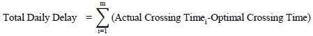
Where,
m = sample size
The definition of optimal crossing time is subject to interpretation by the stakeholders and also depends on the border crossing. For computation purposes, optimal crossing time could be defined as the minimum crossing time observed for a given time period. It can also be defined as a statistical measure such as average crossing time.
Figure 9 shows daily total delay measured at BOTA using minimum crossing time and average crossing time. Total delay is the summation of individual delay of trucks identified by the RFID-based border crossing time and wait time measurement system. The two graphs in Figure 9 show that the total delay is much different depending on whether the optimal crossing time is defined by the minimum crossing time or the average crossing time.
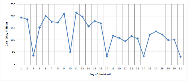
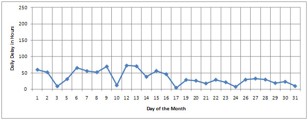
Figure 9. Daily Total Delay of Trucks Measured at BOTA.
If the installed RFID-based border crossing time and wait time measurement system only collects crossing times of a certain portion of the total inbound trucks, then the total delay can be projected to reflect total delay for all inbound vehicles using the following equation:
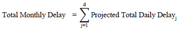
Where,
d = Total number of days RFID collected the data in the month
OR
Average delay per vehicle is an average of extra time spent by all trucks while crossing the border and is a powerful tool in communicating to non-technical audiences. Delay per vehicle is estimated by dividing the total delay by the number of vehicles or sample size during the same time. This normalizes the total delay value, and is important when comparing delay with other border crossings. Figure 10 shows average delay per truck for different days in a month measured at BOTA using minimum and average crossing time as optimal crossing time.
Where,
m = sample size
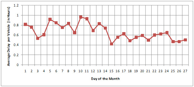
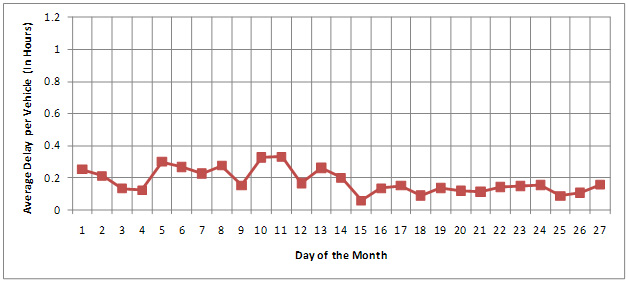
Figure 10. Average Delay per Truck at BOTA.
Determining Length of Peak Periods
Historical and current trends showing increased or decreased length of peak periods are excellent indicators for monitoring congestion and system performance.
It is preferable to use 15-minute average crossing or wait time information over a day to identify peak and off-peak hours. Raw data cannot be used because it is difficult to identify peak from off-peak hours, as there may be several trucks that might take longer than other trucks at the same time and hence show false peaks. Measuring the length of peak periods requires establishing some kind of baseline representing off-peak periods—preferably median value for the entire day. Using a visual method, presence and length of peak periods can be identified, as illustrated in Figure 11. Establishment of peak periods can also be done through stakeholder input. Also, it is entirely possible to develop an automated method to determine peak and off-peak periods for a given data set.
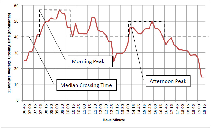
If monitoring the length of peak and off-peak periods becomes difficult to accomplish due to absence of defined peaks and off-peaks, presenting the number of hours the facility operated above the base value is also an excellent mechanism to explain length of congestion at border crossings. This latter value can then be used to make before-after comparisons of performance of border crossings.
Using the logic in Figure 11, the median value is 42 minutes and the number of 15-minute intervals that have an average crossing time higher than 42 minutes is 25 out of 52 total intervals. Hence, the percentage of time periods that exceeded the median values is 48 percent, which is the percentage of time the border crossing operated above the base value (or optimal crossing time) on a typical day.
Determining Percentage of Congested Trips
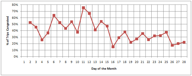
Comparing percentage of congested trips at different time periods indicates trends about performance of a border crossing. Comparisons can also be done before and after improvements are implemented. To define trips as congested, a baseline has to be identified. The baseline preferably is an average crossing time instead of minimum crossing time, which results in almost all the trips operating as congested trips.
To determine percentage of congested trips, a block of raw data either spanning a full day, week, or month for which the analysis is being performed is required. Then the next steps are to:
- Obtain a baseline value of average crossing time for the analysis period.
- Identify the number of trips that had crossing times above the baseline value, and obtain the percentage of total trips that exceeded the baseline.
Figure 12 shows daily variation of percentage of trips that were congested based on the assumption that average crossing time is an optimal crossing time. As noted earlier, stakeholders may choose to establish the crossing and wait time goal for their region as the optimal crossing time.
2 Buffer index is the extra time that is required to cross the border (average) and indicates reliability of the service. Buffer index expresses the amount of extra buffer time needed to be “on time.” ↑
3 The 95th percentile is a widely used mathematical calculation that can be used for border crossing and wait time measurement applications. Simply put, in this context, it refers to the amount of time within which 95 percent of commercial vehicles cross the border from queue to departure in the case of crossing time measurement, or queue to CBP Primary Inspection in the case of wait time measurement. Even though the 95th percentile is widely used, stakeholders can choose different percentiles in place of the 95th percentile. ↑