5. PERFORMANCE MEASURE COMPUTATIONAL PROCEDURES
In this chapter, various procedures used to compute the work zone performance measures of interest are described. Some basic computations must be made once the necessary data is obtained to translate that data into the performance measures of interest. For example, data from point measures of an electronic traffic surveillance system will have actual speeds at several locations, but these must be extrapolated across multiple locations in sequence to estimate travel times and delays. Those speeds must also be compared between point measure locations to determine the estimated length of queue that exists during each time interval of interest. If a travel time-based surveillance system is being used, travel times and delays are being measured directly, but queue lengths must somehow be approximated based on those data. If queue lengths are being collected directly by field inspectors using the manual documentation technique, computations are needed to estimate how travel times may be affected by the length and duration of the queues that are documented. The following sections describe these computational procedures in detail.
POINT MEASUREMENT ELECTRONIC TRAFFIC SURVEILLANCE DATA COMPUTATIONS
It is generally assumed that traffic flow characteristics obtained at a particular point measurement location represent conditions for some distance upstream and downstream of that measurement location. Therefore, a roadway section is divided into a series segments, with conditions in each segment assumed to be represented by its corresponding spot sensor data, as illustrated in Figure 4. The travel time at any point in time j across a region i (TTij) is simply the length of that region (Li) divided by the speed at that point in time obtained from the sensor. Summing the individual travel times for each region together provides a total travel time over the length of roadway of interest at that point in time.
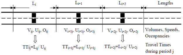
Figure 4. Illustration of Traffic Surveillance Estimates using Spot Sensor Data.
To estimate work zone delays, the travel times estimated in a pre-work zone condition can be directly compared to those estimated from the speeds measured during the work zone over the same summed length of interest, and the difference between the two considered the individual motorist delay being created by the work zone. As an alternative, a desired speed through the work zone can be defined and travel times based on that desired speed used as a baseline to compare against actual work zone travel times. Such an approach might be used if the agency has posted a reduced speed limit through the work zone, and does not want delays measured against the normal, non-work zone speed limit and operating speeds. With individual motorist delays identified, the number of motorists encountering these delays can be multiplied by this individual delay and summed over the duration of the work activity (and eventually, the project) to estimate total delay.
Next, to approximate queue lengths from point measurements, the speeds at each measurement location are examined in sequence and over time to identify regions in which speeds drop below a selected threshold (for 70 mile-per-hour [mph] roadways, a 35 mph speed would be recommended as the threshold denoting queued conditions). The time period when speeds are below the threshold represent the duration of the queue in each point measurement segment. To estimate the length of queue over time, speeds at successive point measurement locations are examined together, and the length Li for each segment denoted as being below the threshold is added together for each time interval of interest.
Figure 5 helps illustrate this process. In this example, point measurements are located 0.2 mile, 0.8 mile, and 1.3 miles upstream of the temporary lane closure. Project diary information indicates that a lane closure began at 9:00 AM and ended at 3:30 PM. The analysis of speeds at the upstream sensor locations indicates that a queue began to develop at approximately 11:30 AM at the first sensor, which grew upstream and reduced speeds at the second sensor at about 12:30 PM. The queue did not extend back to the third sensor, since speeds never did drop below 30 mph at that location during the hours of work activity. Therefore, the queue length each hour would be estimated as shown in Table 7.
| Time | Estimated Location of Upstream End of Queue | Estimated Queue Length |
|---|---|---|
| 11:00 am | None | 0 |
| 12:00 pm | Between Sensors #1 and #2 | 0.2 + (0.6/2) = 0.5 mile |
| 1:00 pm | Between Sensors #2 and #3 | 0.2 + 0.6 + (0.5/2) = 1.05 mile |
| 2:00 pm | “ | 1.05 mile |
| 3:00 pm | “ | 1.05 mile |
| 4:00 pm | None | 0 |
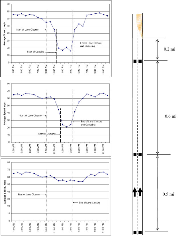
Figure 5. Example of Sensor Speed Analysis to Determine Duration and Length of Queue.
TRAVEL-TIME BASED ELECTRONIC SURVEILLANCE DATA COMPUTATIONS
If travel time information is obtained directly from an electronic surveillance system, the estimation of individual motorist delay over the roadway segment of interest is straightforward. The difference in travel times between normal, non-work zone conditions (at the same time-of-day) and those measured when the work zone is present is the individual motorist delay that exists at that particular time period. Multiplying the individual delays in a given time interval by the number of vehicles passing through the work zone, and accumulated over the days and time periods of interest, yields the total delay (in vehicle-hours) caused by the work zone.
Unfortunately, travel-time based electronic surveillance methods themselves do not also count traffic data. Consequently, volumes occurring through the day (and night) on the roadway segment must be measured by other means (such as temporary traffic counters) or approximated based on historical volumes developed for planning and programming purposes. In many states, only total daily traffic volumes are estimated for most roadway segments. If this is the case, a method of dissecting that 24-hour count into estimated hourly counts by direction will be required. Fortunately, most state agencies have directional and hourly distribution factors developed for various roadway classes that can be used for this purpose. In other locations, nearby automated traffic recording (ATR) stations may be used to generate directional and hourly volume distribution values.
Travel-time based electronic surveillance data is also more limited with respect to estimating queue lengths and durations. If antennae are located close enough together, conditions within each segment may be similar enough to allow for a segment-by-segment comparison as described above for spot sensor data. However, as the length between successive antennae increases, the possibility for missing any queuing that occurs increases. This is because while speeds may drop dramatically in the region where congestion and queuing exists, its effects are diluted with the other portions of the segment that may be operating at higher speeds, either normal (non-work zone) speeds prior to reaching the start of the queue, and/or at speeds near capacity flow conditions through the work zone itself. While it would be mathematically possible to define equations to relate the lengths of the non-work zone, queued, and work zone subsections with a given roadway segment based on assumed or estimated speeds of each subsection, the level of effort required and potential magnitude of errors possible suggest that it would be preferable to simply rely on such data for travel time delays, and to have field personnel manually document queue lengths and durations as described in the next section.
MANUAL QUEUE LENGTH DATA COMPUTATIONS
For locations in which field crew documentation of queue lengths present during a work shift is the primary traffic flow data available, historical estimates of traffic volumes must be obtained as discussed above for travel-time based electronic traffic surveillance systems. In addition, computational methods are needed to estimate how travel times are affected by the presence of the queue.
The manual queue documentation approach will work best if applied at locations when and where, in the absence of the work zone, congested traffic flow conditions would not exist. If this is the case, then the queues as well as the travel times that result because of the queues will be attributable to the work activity in the work zone. Of course, it is possible that an incident or adverse weather conditions in or immediately upstream of the work zone could also contribute to the queue and delays of a work zone. If such incidents occur, it would be important for field personnel to make a special note about it on the data collection form so that the queue and delay numbers can be appropriately interpreted.
To estimate how the documented queues result in travel time delays, it is assumed that both the queue itself and the work zone result in slower speeds for some travel distance. This is depicted in Figure 6. If a queue has formed upstream of the work zone (at the lane closure bottleneck), it is realistic to assume that the flow rate through the work zone is at or near capacity, such that the speed at capacity flow can be assumed to govern through the work zone. For simplicity purposes, an assumption of a linear relationship between speeds and density would suggest that the capacity flow speed would be one-half of the free-flow speed on the facility. Upstream of the work zone, the queue that develops would be flowing at a speed less than the capacity flow speed. Again using a simple linear speed-density relationship, the following equation produces an estimate of the average speed in queue as a function of the normal roadway capacity and the capacity through the work zone (21):
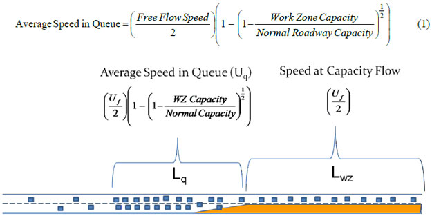
Figure 6. Components of Work Zone Delay.
The capacity of the work zone can be estimated using procedures in the Highway Capacity Manual (HCM) (22). The HCM also provides procedures to estimate the normal traffic-carrying capacity of the roadway segment. For the degree of accuracy being targeted through these computations, the following approximations will usually suffice:
- For 65- and 70-mph roadways: 2200 vehicles per hour per lane * number of lanes on the facility
- For 60-mph roadways: 2000 vehicles per hour per lane * number of lanes on the facility
Assuming that these speeds are maintained, on average, through the entire length of the queue and work zone documented, estimates of average delays per vehicle through the queue can be computed as a function of the length of queue. Some threshold (most likely the desired speed or the posted work zone speed limit [UWZSL]) would serve as the basis against which the longer travel times through the queue would be computed. This queue delay would then be added to the delay that would be generated as vehicles pass through the remainder of the work zone at capacity flow speeds (30-35 mph):
![]() (2)
(2)
Once the average delay per vehicle is estimated for each time interval that a queue is noted on the documentation form, the total vehicle-hours of delay is computed simply by multiplying the normal hourly volume by these average delay values. If the begin and end times of the lane closure and queue do not occur exactly on the hour, extrapolation techniques should be used to estimate the delays during that portion of an hour.
The use of historical volumes for these computations implies that any diversion that occurs because of the work zone will result in delays for diverted motorists that are approximately equal to those being experienced by motorists remaining on the roadway and passing through the queue and the work zone. Such an approximation is likely to be fairly reasonable given the approximate level of accuracy anticipated in the queue length and duration estimation process. If actual traffic counts during the work activity are available, it may still be more appropriate to utilize historical volumes on the facility so that the mobility effects of traffic diversion are taken into consideration to some degree. In general, diversion concerns will only exist in urban areas where there are frequent access and egress points to a roadway, and multiple alternative paths to use as diversion routes. In rural areas, the options are much more limited, and most traffic will have to pass through the queue and work zone.
previous | next