5.0  Calibration

Upon completion of the error checking step, the analyst has a working model.  However, without calibration, the analyst has no assurance that the model will correctly predict traffic performance for the project.  Calibration isthe adjustment of model parameters to improve the model’s ability to reproduce local traffic conditions.

CORSIM cannot be expected to perfectly match all possible real-world conditions and situations.  CORSIM was designed to be flexible enough that an analyst can correctly calibrate the network to match the local real-world conditions at a reasonably accurate level.  For the convenience of the analyst, CORSIM provides default values for the model parameters.  However, only under rare circumstances will the model be able to produce accurate results for a specific area using only the default parameter values. 

Therefore, the importance of calibration cannot be overemphasized.   Calibration is a required step during a traffic analysis to ensure the model can reproduce localdriver behavior and traffic performance characteristics, and calibration should always be done prior to evaluating alternatives.  Regardless of the size or complexity of the network, the analyst should always perform some level of calibration tests to ensure that the coded model accurately reproduces local traffic conditions and behavior.

5.1 Objectives of Calibration

The fundamental assumption of calibration is that the travel behavior models in the simulation model are essentially sound.  There is no need to verify that they produce the correct delay, travel time, and density when they are given the correct input parameters for a link.  It is the software developer’s job to perform verification by checking the accuracy of the software implementation.  It is also the software developer’s job to perform validation of the model to ensure it produces data that is consistent with a wide range of real-world applications. 

CORSIM comes with a set of user-adjustable parameters for the purpose of calibrating the model to local conditions.  Therefore, the objective of calibration is to find the set of parameter values for the model that best reproduces local traffic conditions.

5.2 Calibration Approach

The calibration approach provided in this guide is based on the same approach recommended in Volume III.  Due to the nature of calibration, an analyst can end up in a circular process that seems to be never-ending.  Fixing one problem may lead to new problems occurring somewhere else in the model.  For this reason, the calibration process needs to be practical, logical, and sequential. 

Volume III identified a basic strategy that is summarized in Figure 45.  The process begins by identifying the calibration MOEs and targets (i.e., thresholds where the differences between the field and model MOEs are acceptable).  Once the calibration MOEs and targets are established, calibration should be performed in three basic steps:

• Calibrate capacity at key bottlenecks:  This is an initial calibration of the capacity of key bottlenecks in the study area.  These bottlenecks will be responsible for the majority of congestion (and thus delays and queuing) in the model.  If the model cannot match the capacity at these bottlenecks, then the system performance MOEs will be nearly impossible to calibrate later in the process.
• Calibrate traffic volumes:  CORSIM internally converts entry volumes and turning percentages into origin-destination percentages and then assigns routes for vehicles.  This conversion results in a good approximation of volumes on small or linear models; however, discrepancies in link and turning movement volumes can occur for larger models with multiple routes possible between origins and destinations.  In these cases, calibration of traffic volumes will be needed to ensure that the model volumes throughout the study area match those in the field. 
• Calibrate system performance:  The overall model MOEs of interest that are used to measure system performance are calibrated in this step.  Typical system performance MOEs include speed, density, travel time, delay, and queues.  This step ensures that the model as a whole reasonably matches the local conditions.

Within each of these steps, real-world MOEs measured in the field are compared to the MOEs estimated by CORSIM and, if they do not meet the established targets, then the model parameters are systematically adjusted until an acceptable match is found.  This process continues through each of the three basic steps until all calibration targets have been met.  Once the calibration targets have been met, then the model represents a close match to field conditions and the analyst is ready to move to the alternative analysis phase of the project.  The following sections of this chapter provide more detail for each of the steps shown in Figure 45.

 

Figure 45 . Flowchart. Calibration approach.

 

As in the other tasks of the analysis process, it is important to manage and document the calibration process.  For example, issues such as who made adjustments to the base model, what adjustments were made, where in the model the adjustments were being made, and why the adjustments were made should all be documented.  Remembering who changed a default value from 1.8 to 1.9 and why that value was changed will be difficult six months after the calibration is complete.  Maintaining control over the base network files and providing proper documentation of the calibration process will eliminate such questions.  Documentation summarizing the calibration process and justification for the calibration adjustments, such as supportive MOE statistics that document how the calibration process provided a closer match to field conditions, should be included as part of the final report and possibly an interim technical memorandum.

5.3 Establish Calibration MOEs and Targets

Before starting the process of calibration, it is important to select which MOEs to calibrate and target thresholds for those MOEs.  Establishing calibration MOEs and targets upfront allows consensus to be built by all parties involved on the degree of error allowed in the calibration process and, as well, provides a “blueprint” for which MOEs to focus on and at which point to stop the calibration process. 

5.3.1  Selection of Calibration MOEs

CORSIM accumulates and calculates hundreds of MOEs.  Some of these MOEs can be measured in the real world, such as average speed and traffic volumes.  Other MOEs, such as fuel consumption and vehicle emissions, are very difficult and expensive to measure in the real world.  System-wide MOEs, such as vehicle-miles traveled (VMT) and vehicle-hours traveled (VHT), are another example of MOEs that are difficult and expensive to collect in the field.  Overall, the selection of MOEs for calibration is limited to those that can be practically collected in the field and are accumulated and reported in CORSIM.  Even if the MOE is the critical MOE used in the alternatives analysis, if it cannot be measured in the field, then it cannot realistically be included as a calibration MOE. 

Capacity MOEs

The first step in the calibration process is to calibrate the capacity at key bottlenecks.  CORSIM, like other microsimulation models, does not output a number called “capacity.”  Rather, the capacity can be estimated by measuring the maximum throughput at the bottleneck location.  The throughput should only be collected when a queue is continually present upstream of the bottleneck, as this is the only time when throughput can be used to determine the capacity of a given location.  Measuring the throughput downstream of a queue is sometimes referred to as the queue discharge rate, which is often slightly lower than the maximum flow rate before flow “breakdown” (i.e., when traffic flow transitions from uncongested to congested conditions).  For calibration purposes, it is recommended to use the queue discharge rate as the capacity MOE for freeway bottlenecks, rather than maximum flow before breakdown, because the discharge rate is more stable and much easier to measure in the field.  Section 2.4 of this volume, along with section 5.3.2 of Volume III,⁽⁷⁾ discusses measuring capacity in the field in more detail.  In CORSIM, the capacity on freeways can be measured using the “Vehicles Out” MOE for the link immediately downstream of the bottleneck location, so long as there is a continuous queue upstream of the bottleneck for the measurement period.

On surface streets, bottlenecks are most often located at traffic signals and stop-controlled intersections.  The capacity of an approach at a traffic signal is directly related to the discharge headway at the stop line (the capacity is a function of the discharge headway and the proportion of effective green time given for that approach).  Section 2.4 of this volume, along with sections 5.3.1 and 5.3.2 of Volume III,⁽⁷⁾ discusses measuring capacity at intersections in more detail.  In CORSIM, the “Vehicles Discharged by Lane” MOE can be used to estimate the model capacity, so long as there is a continuous queue upstream of the intersection approach of interest for the measurement period.     

Traffic Volume MOEs

The second step in the calibration process is to calibrate the traffic volumes, which consists of ensuring that the link and turning movement volumes in the CORSIM model match the field traffic counts.  On freeways, “Vehicles In,” “Vehicles Out,” and “Volume” are all reported on individual links by CORSIM.  On surface streets, “Average Volume” and “Vehicles Discharged by Lane” are reported on individual links by CORSIM.  “Vehicle-trips” is reported for each turning movement on CORSIM surface streets.  Any of these MOEs can be used to calibrate field measured volumes, as long as the field measurement is defined and measured similarly to the MOE used in CORSIM.  For example, a 15-minute average turning count at an intersection is a typical field measurement.  To calibrate this measured volume, an analyst would need to obtain a 15-minute average of the “Vehicles Discharged by Lane” for the particular turning lane from the CORSIM output, taking care not to obtain the cumulative count over the entire simulation period.

System Performance MOEs

The third, and likely most difficult, step in the calibration process is to calibrate the system performance of the model.  Types of MOEs to use in the system performance calibration include speed, density, travel time, delay, stops, and queues.  CORSIM measures all of these types of MOEs, often in many different forms.  For example, CORSIM measures the “Delay Time,” “Stopped Time,” “Queue Delay,” and “Control Delay” on surface street links, expressed in seconds per vehicle.  The key is to select the delay MOE for calibration which matches how delay was measured in the field.  This will ensure an “apples-to-apples” comparison between field and model MOEs.  For example, if stopped time was collected in the field, then the “Stopped Time” MOE should be used in CORSIM for system calibration. 

The scope of the analysis will also help define the system performance calibration MOEs.  For example, if the purpose of the analysis is to test different bus route alternatives, the calibration MOEs should include MOEs related to bus routing.

5.3.2  Establishing Calibration Targets

Once the calibration MOEs have been selected, the project team should then establish calibration targets for these MOEs.  The objective of model calibration is to obtain the best match possible between model and field measurements of MOEs.  However, there is a limit to the amount of time and effort anyone can put into eliminating error in the model.  There comes a point of diminishing returns where large investments in effort yield small improvements in accuracy.⁽⁷⁾  The purpose of setting calibration targets is to set a stopping point for fine-tuning the calibration and consider the model calibrated.

There are no standards on acceptable calibration targets, as the targets will likely vary according to the size of the model, resources available, the purpose and objectives of the project, and the types of decisions that will be made from the simulation analysis.  For example, large simulation models will probably have less stringent targets than small models due to the difficulty in matching MOEs for all links in a large, complex network.  Also, using the simulation analysis to test finely-tuned signal optimization plans will require more stringent targets than using the model for determining the number of freeway lanes needed.

Calibration targets can be relatively straight-forward, such as having a target of all model MOEs for all network links being within 10 percent of the field MOEs.  Such a simple calibration target plan is best suited for small, straight-forward modeling projects.  However, for larger models, a more sophisticated set of targets may be necessary; in particular, a set of targets that acknowledges that it will be very difficult to ensure all links within the network will meet the target.  For larger networks, it is important to focus on matching MOEs at critical locations in the network (i.e., bottleneck locations or locations where roadway improvements are being considered), as many hours can be wasted on calibrating portions of the network that will not have an impact on the final results or recommendations. 

Table 11 provides an example of calibration targets that were developed by Wisconsin DOT for their Milwaukee freeway system simulation model.⁽⁷⁾  They are based on guidelines developed in the United Kingdom.⁽¹³⁾  These targets acknowledge the difficulty in matching all links in the network to field conditions, as the targets ensure that at least 85 percent of the links are within a target percentage or value of the field conditions.  This table is provided merely as an example, as the calibration targets should be tailored to the specific analysis at hand.  As mentioned previously, the calibration targets will likely vary depending on factors such as the size of the model, resources available, purpose and objectives of the analysis, and types of alternatives analyzed.  The project team should develop consensus on specific calibration targets before proceeding with the calibration effort.

 

Table 11. Wisconsin DOT freeway model calibration targets. ⁽¹⁴⁾

MOE Criteria	Calibration Acceptance Targets
Hourly Flows, Model versus Observed
Individual Link Flows
< 700 veh/hr	Within 100 veh/hr of Field flow for > 85% of cases
700 to 2,700 veh/hr	Within 15% of Field flow for > 85% of cases
> 2,700 veh/hr	Within 400 veh/hr of Field flow for > 85% of cases
Sum of all link flows	Within 5% of sum of all link counts
GEH Statistic* for individual link flows	GEH < 5 for > 85% of cases
GEH Statistic for sum of all link flows	GEH < 4 for sum of all link counts
Travel Times, Model versus Observed
Journey Times, Network	Within 15% (or 1 min, if higher) of > 85% of cases
Visual Audits
Individual Link Speeds	Visually acceptable speed-flow relationship to analyst’s satisfaction
Bottlenecks	Visually acceptable queuing to analyst’s satisfaction

 

where:             E = model estimated volume
                                    V = field count

Figure 46 . Equation. Calculating the GEH Statistic. ⁽¹⁴⁾

 

Another example of suggested calibration targets is “Theil’s Inequality Coefficient,” which is broken down into three parts, each of which provides information on the differences between the model measures and the target measures.  Further discussions on Theil’s Inequality Coefficient can be found in the Advanced CORSIM Training Manual⁽²⁾ and in Hourdakis, Michalopoulos, and Kottommanil.⁽¹⁵⁾

5.4 CORSIM Run Considerations

The calibration approach described in this chapter requires the analyst to run, or apply, CORSIM for the existing or baseline conditions many times, until the model MOEs adequately match the field (real-world) MOEs.  The CORSIM User’s Guide describes in detail the steps required to run CORSIM.  The purpose of this section, however, is to discuss some key issues that the analyst should consider when running CORSIM during the calibration step. 

5.4.1  Multiple CORSIM Runs

Due to the stochastic nature of CORSIM, the results from individual runs can vary by 25 percent and higher standard deviations may be expected for facilities operating at or near capacity.  Thus, it is necessary to run CORSIM multiple times with different random number seeds to gain an accurate reflection of the performance of the model.  The CORSIM Driver Tool has a built-in multiple-run capability and a built-in output processor that collects statistics from each run and summarizes them.  The multi-run capability runs a test case multiple times, changing the random number seeds for each run.  Refer to Appendix D for more information on the usage of random seed values in CORSIM.  The output processor collects user-selected MOE data for selected links from CORSIM over multiple runs and organizes the data into a single summary file.  When output processing is selected, a statistics file (or files, depending on how many formats are selected) is created.  These files are overwritten if they already exist, and are created if they do not exist.  The benefits of using the multi-run feature include:

• Data from multiple runs are automatically summarized based on user-selected MOEs and statistics, eliminating unnecessary time and errors that could be made in manually compiling statistics from multiple runs.
• The feature is very flexible in that it allows the analyst to select just one, or all, of the MOEs to summarize statistics across multiple runs.
• The analyst can select from a wide range of summary statistics to be automatically calculated based on the selected MOEs, such as the mean, median, standard deviation, and 95th confidence interval.
• Use of the tool encourages analysts to account for the stochastic nature of CORSIM.

When the base model is satisfactory, the number of runs has been set, and MOE selection is complete, the model should be run multiple times using the CORSIM multi-run feature.  When all runs are finished, the output processing will write data to the selected file types.  This may take some time depending on the size of network, length of run, number of MOEs selected, number of network objects selected, and number and type of statistical processing. 

After the multiple runs of CORSIM have been completed, the analyst should review the output to verify that all of the individual runs finished correctly.  Under certain circumstances, the CORSIM simulation may encounter exceptional conditions and be unable to complete a run.  If this happens, statistical data for that run will be discarded and will not factor into the analysis functions (such as Mean and Standard Deviation).  The analysis functions will be applied as if that run had not occurred.  Refer to the CORSIM User’s Guide for more information on setting up and starting multiple runs of CORSIM.

Determining the number of times to run the simulation depends on two primary variables: the variance in the mean of one or more MOEs, and the tolerable error as selected by the analyst.  The sample size required for the selected tolerable error calculates the minimum number of simulation runs (i.e., the sample size) required to produce results with a “sampling error” less than or equal to the tolerable error entered by the user.  The formula for the sample size calculation is:

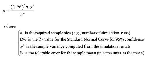
Figure 47. Equation. Determining the appropriate number of simulation runs to complete.

 

The CORSIM output processor can calculate how many runs are necessary to achieve results that are within the tolerable error.  Refer to the “Formats and Options” dialog in the CORSIM User’s Guide⁽¹⁾ for information on selecting the option to calculate the required number of runs.  In order to calculate the number of runs, a preliminary set of runs must be made.  Twenty runs should produce enough variance to calculate a reasonable number of runs for the statistical analysis.

5.4.2  Simulation Time Frame

The time frame to simulate should have been decided in the scope of the project (chapter 1) so that the data collection (chapter 2) would be based on that time frame.  Prior to this stage in the model development process (chapter 3), a short simulation time may have been used for error checking.  Make sure the start time and duration of the simulation reflect the period designated in the scope of the project and represented in the demand data.

5.4.3  Exclusion of Initialization Period

The artificial period where the simulation model begins with zero vehicles on the network (referred to as the “initialization period” or “fill period”) must be excluded from the reported statistics for system performance.  CORSIM will do this automatically.  The initialization period typically ends when equilibrium has been achieved.  Equilibrium is achieved when the number of vehicles entering the system is approximately equal to the number leaving the system.  The algorithm used by CORSIM does not work properly in all circumstances.  For example, if the data collected during a run shows a sharp decrease in value soon after the initialization period, it is a good indication that equilibrium was not reached.  Thus, the analyst should check the CORSIM output data to ensure equilibrium has been reached in the CORSIM run.  Model output should not be used if equilibrium has not been reached, as the results will not represent the actual volumes attempted to be modeled.  Appendix C has a more in depth discussion of the initialization period.

5.4.4  Link Aggregations into Sections

CORSIM can treat a particular set of links as a single entity for the purpose of computing significant MOEs over multiple links.  Each such set is known as a “link aggregation” or “section” and is identified by a user-defined section number.

Any surface links within the network can be specified as part of a section; however, the links do not have to form a continuous path through the network.  It is possible to aggregate any set of links into a section.

When this option is selected, an additional output table is provided within each standard cumulative output.  This table presents aggregated statistics for each section identified.  The full set of statistics is still provided for each link individually in the link statistics table.

5.5 Calibrate Capacity at Key Bottlenecks

As shown above in Figure 45, calibrating the capacity at key bottlenecks is the first step in the calibration process.  Having a CORSIM model that can replicate the location and severity of bottlenecks in the field is a crucial initial step in calibration, as these bottlenecks will be responsible for the majority of congestion throughout the network.  Thus, if the model cannot replicate the throughput at bottlenecks, then it will be very difficult to calibrate the system performance MOEs later in the calibration process.

This step is performed by evaluating a few key points in the network and adjusting the model parameters in a systematic manner until the throughput volume just downstream of these bottlenecks can be matched between the field and model.  As mentioned earlier in section 5.3, it is recommended to measure the queue discharge rate downstream of the bottleneck as the measure of capacity, rather than the maximum flow before breakdown (which is typically slightly higher than the queue discharge rate) because the discharge rate is more stable and much easier to measure both in the field and in CORSIM.  Figure 48 shows some typical bottleneck locations on freeways.

If the model does not initially show congestion at the same bottleneck locations as exist in the field, then the demands coded in the model should be temporarily increased to force the creation of congestion in the model at those bottlenecks.  These temporary increases should be removed after the capacity calibration has been completed.  On the other hand, if the model initially shows congested bottlenecks at locations that do not exist in the field (i.e., false bottlenecks), it will be necessary to increase the capacity of the model at these points to remove the false bottleneck from the model.

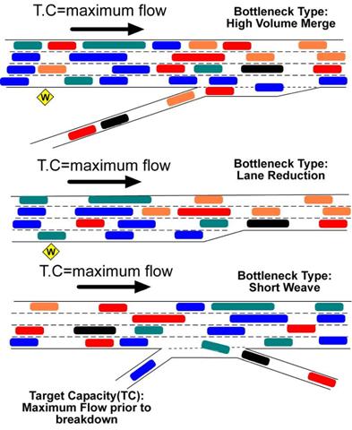
Figure 48 . Illustration. Typical freeway bottleneck locations.

5.5.1  Freeway Capacity Calibration

There are many parameters in CORSIM that affect the freeway capacity, so it is important to narrow the list to a few parameters that are the most sensitive to capacity.  A recent sensitivity test was completed on all CORSIM parameters relating to driver behavior logic.  This test is documented in the report entitled, Identifying and Assessing Key Weather-Related Parameters and Their Impacts on Traffic Operations Using Simulation.⁽¹⁶⁾  Based on this study, and past experiences with real-world simulation studies, the candidate list of key parameters to adjust for calibrating freeway capacity include:

• Car following sensitivity factor – This is a global parameter that affects all freeway links.  This value represents the primary factor in calculating the desired time headway (in seconds) between a leader-follower pair.  A higher value means more space between vehicles and thus a lower capacity.  Each driver type has a different value (ranges from 1.25 seconds for conservative drivers to 0.35 seconds for aggressive drivers, with a mean value of 0.80 seconds).
• Car following sensitivity multiplier – This parameter can be adjusted for each individual link and represents a multiplier of the car following sensitivity factor.  The default value is 100 percent; thus increasing this value for a specific link to 110 percent (as an example) would increase the individual car following sensitivity factor for each driver type by 10 percent on that link.  Increasing this value means more space between vehicles and thus a lower capacity.
• Lag acceleration and deceleration time – These are global parameters (acceleration and deceleration time are two separate parameters) that affect all freeway links.  These values represent the time delay due to perception/reaction time for drivers when starting to accelerate or decelerate.  A higher value for these parameters means slower reactions, which translates to a lower capacity.  The default values for these parameters are 0.3 seconds.
• Pitt car following constant – This is a global parameter that affects all freeway links.  This value represents the minimum distance between the rear of the lead vehicle and front of the following vehicle.  A higher value for this parameter means more space between vehicles and thus a lower capacity.  The default value is 3.05 m (10 ft).

These parameters are directly related to the car following logic within FRESIM.  There are also 10 parameters related to the lane changing logic within FRESIM; however, altering these parameters is typically not worthwhile because they are not very sensitive to aggregate measures (i.e., 15-minute averages) of throughput.⁽¹⁶⁾

Table 12 shows an example of adjusting the car-following sensitivity factor in an attempt to increase the freeway capacity.  In this example, the default values for each driver type were decreased by 10 percent, which will create less space between vehicles and thus increase the capacity.  Note that decreasing all driver type values by 10 percent is equivalent to decreasing the “Car following sensitivity multiplier” for all freeway links on the network by 10 percent.

 

Table 12 . Example adjustment of the car-following sensitivity factor.

Case	Driver Type
	1	2	3	4	5	6	7	8	9	10
Default	1.25	1.15	1.05	0.95	0.85	0.75	0.65	0.55	0.45	0.35
10% Decrease	1.13	1.04	0.95	0.86	0.77	0.68	0.59	0.5	0.41	0.32

 

Out of the parameters described above, the “Car following sensitivity factor” and link-level multiplier of that factor are the most sensitive to changes in the default values when attempting to alter the capacity at a bottleneck.  Figure 49 shows an example of the sensitivity of throughput to changes in the “Car following sensitivity multiplier.”  The test network for this figure was a basic freeway segment with three lanes.  The maximum throughput on the segment represents the capacity of the segment.  As shown in the figure, increasing the “Car following sensitivity multiplier” for the freeway link results in a proportional decrease in capacity.  Increasing the multiplier from 100 to 125 results in an approximately nine percent decrease in capacity (from 2,200 to 2,000 veh/h/ln).

 

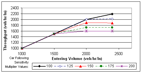
Figure 49 . Figure. Example of sensitivity of car following sensitivity
multiplier on throughput of a basic freeway segment.

 

Attempts to match field-measured bottleneck capacity should first focus on the key global parameters, starting with the “Car following sensitivity factor” and then the “Lag acceleration and deceleration time” and “Pitt car following constant.”  Attempts to increase the freeway capacity on the network would require decreasing the values of these parameters from their default values.  While it is possible to just focus on link-level parameters such as the “Car following sensitivity multiplier”, a global adjustment ensures the accuracy of the capacities on all links (even those not currently congested), rather than only those on specific links.

In cases where there are multiple freeway bottlenecks, some of which require the model capacity to be increased and others which require the model capacity to be decreased, then adjusting the global factors by themselves will not be sufficient.  In this case, the link-level “Car following sensitivity multiplier” value may need to be adjusted separately for each bottleneck calibration.  This link-level calibration may be needed when the bottleneck is due to a local condition not present in the remainder of the network, such as a horizontal curve, vertical curve, or narrow lanes.

In addition to the key parameters listed above, many of the input values entered in the base model development step (chapter 3) also have an impact on capacity, such as the percentage of trucks; origins and destinations within weaving areas; and the placement of warning signs for anticipatory lane changes, exit ramps, and lane drops.  The values entered for these parameters should be entered in the base model development step based on field data collection and, thus, should be known and set values.  However, if the key parameters listed above do not have the desired impact in calibrating capacity, then slight modifications to these additional capacity-altering parameters may be warranted. 

For example, when CORSIM vehicles cross warning sign “reaction points”, vehicles begin to react to downstream conditions or begin to target a new lane (e.g., targeting an exit ramp or moving away from a lane drop).  Refer to chapter 3 of this volume, or the CORSIM User’s Guide, for more information on warning sign parameters.  In general, moving these warning sign locations further upstream will result in smoother, less turbulent lane changing conditions and can thus increase the capacity of a bottleneck.

5.5.2  Surface Street Capacity Calibration

As mentioned previously, surface street bottlenecks are primarily created by traffic signals or stop-controlled intersections and, thus, capacity calibration on surface streets should focus on a few key intersections.  The candidate list of parameters to adjust for calibrating the capacity of signalized and stop-controlled intersections includes:

• Mean discharge headway – This is a link-level parameter that represents the mean headway between vehicles discharging from a standing queue.  The default value is 1.8 seconds.  Increasing this value will result in a decrease in capacity.  This parameter is useful in calibrating the capacity of signalized intersections.
• Mean startup delay – This is a link-level parameter that represents the mean delay due to perception/reaction time of the first vehicle in a queue due to a traffic signal.  The default value is 2.0 seconds.  Increasing this value will result in a decrease in capacity.  This parameter is useful in calibrating the capacity of signalized intersections.
• Acceptable gap in oncoming traffic (left turns and right turns) – These are global parameters (left turns and right turns have separate parameters) that represent the acceptable gap in crossing traffic that a vehicle will accept while making a permitted left turn or a right turn on red (RTOR) at a traffic signal.  Each driver type has a different value (the left turn values range from 7.8 seconds for conservative drivers to 2.7 seconds for aggressive drivers, with a mean value of 5.0 seconds).  Increasing these values will result in vehicles waiting longer at signals and thus lowering the capacity for these movements.
• Cross-street acceptable gap distribution (near-side and far-side) – These are global parameters that represent the acceptable gap in crossing traffic that a vehicle will accept while at a stop sign.  Each driver type has a different value (the near-side values range from 5.6 seconds for conservative drivers to 2.0 seconds for aggressive drivers, with a mean value of 3.8 seconds).  Increasing these values will result in vehicles waiting longer at stop signs and thus lowering the capacity of the approach.  Vehicles at yield-controlled intersections will subtract 1.5 seconds from these values to calculate their acceptable gap in crossing traffic.

For calibrating signalized intersection approaches, the capacity is most sensitive to the “Mean discharge headway” parameter and, thus, attempts at calibration should focus first on this parameter, followed by the “Mean startup delay” parameter.  Figure 50 shows an example of the sensitivity of throughput to changes in the “Mean discharge headway.”  The test network for this figure was a fully-actuated signal with two through lanes and a separate left turn lane with a protected left turn phase.  The maximum throughput on the segment represents the capacity of the segment.  As shown in the figure, increasing the “Mean discharge headway” for the approach link results in a proportional decrease in capacity.  For example, increasing the value from 1.9 to 2.2 seconds results in an approximately 12 percent decrease in capacity (from 5,180 to 4,540 veh/h).

 

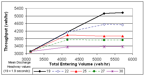
Figure 50 . Figure. Example of sensitivity of mean discharge headway on
throughput of a signalized intersection approach.

 

The distribution of discharge headway and startup delay can be edited on a global scale using the distribution codes by driver type for these two parameters.  However, changing the distribution of these values is not recommended because a recent sensitivity test of these distributions showed that they are not sensitive to aggregate MOEs such as 15-minute averages of throughput, speed, and/or density.⁽¹⁶⁾

Another consideration in the calibration of signalized intersection approaches is that the green time given to the approach in the model matches that in the field.  The green time for the approach directly affects the capacity of the approach, so ensuring the model is consistent with the field will make this calibration effort much easier.  For actuated signals that are operating at or over capacity, this can simply be done by checking that the maximum green time coded in the model matches that in the field. 

The parameters related to acceptable gap listed above are only adjustable on a global scale; thus, calibrating individual stop-controlled or permitted left-turn movements is not possible in the most recent version of TSIS/CORSIM (version 6.0) without changing the values for all movements in the network.  As stated previously, the primary focus of capacity calibration should be on the key bottlenecks in the network, as they will directly impact the performance of the overall network.  Thus, the analyst should still use these global parameters in the calibration of any bottlenecks related to stop, yield, or permitted left-turn movements.  The performance of the entire system will be calibrated in the final calibration step, giving the analyst an opportunity to calibrate other portions of the network impacted by these global parameters.  

In congested networks with closely-spaced intersections or a grid pattern of surface streets, bottleneck capacity could be impacted by weaving on roadway sections due to short lane-changing areas or queues that spillback and block upstream intersections.  In these cases, the analyst should consider calibrating parameters such as “Spillback probabilities” and “Time to react to sudden deceleration of lead vehicle.”  These parameters are discussed in more detail in section 5.7. 

5.6 Calibrating Traffic Volumes

As shown above in Figure 45, calibrating the traffic volumes is the second step in the calibration process.  This step is only needed if the model includes parallel streets or a network of streets with multiple routes possible within the model.  The purpose of this step is to ensure that the model volumes throughout the study area match those in the field.  Having a CORSIM model that can replicate the traffic volumes in the field is a crucial step in calibration, as the traffic volumes directly impact the performance of the entire network.  Thus, if the model cannot replicate the traffic volumes in the field, then it will be very difficult to calibrate the system performance MOEs later in the calibration process.

This step is performed by comparing the link and turning movement volumes throughout the model to those measured in the field (not a future forecasted volume), and then adjusting the model parameters in a systematic manner until the volumes in the model match those in the field to an acceptable degree as established in the calibration targets (section 5.3).  At this point in the modeling process, it is assumed that the field volumes were entered into CORSIM correctly without any errors, and that any discrepancies between field and model volumes are due to how CORSIM routes vehicles through the network. 

Typically, the analyst should calibrate the model volumes to all traffic counts in the field.  However, for very large networks this may not be feasible and, in these cases, the analyst should focus on calibrating the volumes at all critical locations in the network (e.g., bottlenecks and congested locations).

5.6.1  Freeway Traffic Volume Calibration

As described previously in section 3.3, the most direct and common method of entering traffic volumes for freeways is by using entering volumes at entry nodes and turning percentages at off-ramp locations.  CORSIM then internally converts these values into origin-destination percentages (i.e., percentage of traffic between each entry node and off-ramp location) using a gravity model (see the CORSIM User’s Guide⁽¹⁾ for more information).  CORSIM does not route vehicles dynamically based on network conditions (e.g., avoiding areas of congestion), and there are no user-editable parameters that affect the internal calculation of origin-destination percentages.  However, unless there are multiple freeways being modeled with more than one possible freeway path between origin and destination, the traffic volumes on individual freeway links should be consistent with those entered into the model.  

If the network does consist of multiple freeways with more than one possible freeway path between origin and destination, then the analyst could manually enter a complete origin-destination table via Record Type 74 to minimize discrepancies in link-level volumes due to CORSIM’s internal origin-destination calculations.  Refer to the CORSIM User’s Guide⁽¹⁾ and section 3.3 of this document for more information on this method.

At a local scale, volumes entering and exiting the freeway at adjacent interchanges may need to be calibrated.  For example, some percentage of freeway on-ramp traffic may exit at the next downstream off-ramp which may not match those calculated by the internal CORSIM gravity model.  In this case, partial origin-destination data may be entered to “override” the CORSIM calculated origin-destination percentages.  Refer to the CORSIM User’s Guide and section 3.3 of this document for more information on this method.

5.6.2  Surface Street Traffic Volume Calibration

As described in section 3.3, the most direct and common method of entering traffic volumes for surface streets is by using entering volumes at entry nodes and turning percentages at intersections.  Thus, each vehicle entering the network will be assigned a path based on the turning percentages encountered at each intersection.  This method results in a good approximation of the volumes on small or linear surface street networks with few route choices available within the network. 

However, the volumes on larger networks or those with a grid-type layout will be more difficult to calibrate because of the various possible routes.  One possible method to better control the volumes on specific segments of the network is to use conditional turn movements.  As described in section 3.3, conditional turn movements allow the user to define turn percentages that are conditional based on the entry movement (i.e., which direction the vehicle entered the link).  Conditional turn movements are useful for closely-spaced intersections, such as at a diamond interchange or offset T intersection, where unrealistic weaving and queuing may occur if the correct volumes are not modeled.

Another method possible for calibrating surface street volumes is when a multi-level urban interchange is present.  If this is the case, then origin-destination data through the urban interchange can be coded rather than turn percentages for each link.  Refer to the CORSIM User’s Guide and section 3.3 of this document for more information on this method.

A final method that may be useful for calibrating traffic volumes on complex surface street networks is to specify an origin-destination table for the entire network via Record Type 176.  As explained in the CORSIM User’s Guide and section 3.3 of this document, specifying an origin-destination table in NETSIM has limitations, such as the specification that only NETSIM links can be coded and that the traffic assignment algorithm is not entirely accurate when actuated control traffic signals are present, so care should be taken in using Record Type 176 and acknowledging its limitations.

5.7 Calibrating System Performance

In the third, and likely most difficult, step of calibration, the overall traffic performance predicted by the fully functioning model is compared to the field measurements of the system, such as speed, density, travel time, and queue lengths.  At this stage, the capacities of the key bottlenecks and the traffic volumes throughout the network have been calibrated; thus, the system performance MOEs from the model should be fairly close to those measured in the field.  However, additional calibration will likely still be needed.

This step is performed by comparing the system MOEs measured in the field to those from the model and adjusting the model parameters in a systematic manner until the system MOEs in the model match those in the field to an acceptable degree as established in the calibration targets (section 5.3). 

Figure 51 shows an example of comparing the field measured average speed to that estimated by the model on a section of freeway.  As shown, the speed profile changes on each segment of the freeway and, while not shown in the figure, the speed profile also changes temporally (i.e., a different speed profile could be graphed for each 15-minute interval).  Thus, comparing the field MOE to model MOE is more complex than just comparing two numbers to each other.  Employing graphical and spreadsheet techniques to compare MOEs over time and space can be useful in the calibration process.  Chapter 6 shows some examples of how to visualize and compare simulation output.  

Viewing the animation of CORSIM runs in TRAFVU can be a useful qualitative tool when calibrating the system performance.   For example, using TRAFVU to view the progression of vehicles in a coordinated set of traffic signals on an arterial can help verify the accuracy of the progression in CORSIM as compared to the field.  The quality of platoon progression can have a significant impact on the system performance (e.g., delays, speeds, and stops) in CORSIM; thus, ensuring the platoon progression is realistic is important.

 

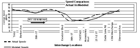
Figure 51 . Figure. Example of comparing actual speed from field to modeled speed.

 

5.7.1  Freeway System Performance Calibration

There are many parameters in CORSIM that affect the freeway system performance, so it is important to narrow the list to a few parameters that are the most sensitive to system MOEs.  A candidate list of parameters to adjust for calibrating freeway system performance includes:

• Car following sensitivity factor, Car following sensitivity multiplier, Lag acceleration and deceleration time, and Pitt car following constant – As described above in section 5.5, these parameters affect freeway capacity and, as a result, also affect system performance.  Increasing these parameter values will have the effect of degrading the system performance MOEs.  The “Car following sensitivity factor” and “Car following sensitivity multiplier” are the most sensitive of these parameters and, thus, are the most effective for calibrating the system performance MOEs.  However, if these parameters were already calibrated in the bottleneck capacity step, then they should be altered here at a minimum level, if possible, to avoid undoing the capacity calibration done earlier.
• Time to complete lane change – This is a global parameter that represents the time to complete a lane change maneuver.  The default value is 2.0 seconds.  Increasing this value results in more extended, smooth lane changes and, thus, generally improved system performance.  Based on a recent CORSIM sensitivity test, this is the only one of FRESIM’s 10 lane changing parameters that have a consistent and moderate impact on system performance MOEs.⁽¹⁶⁾ This parameter may be helpful in calibrating freeway sections with a high frequency of lane changing, such as weaving sections or closely-spaced interchanges, where the lane changing activity is affecting the system performance.
• Mean free-flow speed – This is a link-level parameter that represents the desired mean speed of vehicles in the absence of any impedance due to other vehicles or traffic control devices.  Each driver type has a different free-flow speed based on a global multiplier (ranges from 88 percent for conservative drivers to 112 percent for aggressive drivers).  Changing the distribution of free-flow speed by altering the global multipliers is not recommended because a recent sensitivity test showed that changing the distribution resulted in inconsistent and occasionally unrealistic impacts on system performance MOEs.⁽¹⁶⁾

The mean free-flow speed should be used for system performance calibration when the model cannot match field conditions at low levels of congestion, as the parameter is intended to model speeds at free-flow conditions.  For example, freeway segments that have a tight horizontal curve, steep vertical curve, or narrow lanes, or alternatively attempting to model adverse weather conditions, may cause degraded system performance during low congestion based on more conservative driver behavior occurring in these conditions.  Ideally, the free-flow speed was measured in the field and entered into the model in the base model development step (chapter 3); however, other driver behavior changes may be occurring during low congestion that are not easily measurable but can be approximated using the free-flow speed parameter.  

For congested conditions, the other parameters mentioned above are better suited for calibration than free-flow speed.  However, it is important to understand that altering the free-flow speed in CORSIM will likely change the average speed for a wide-range of volume conditions all the way up to the point of maximum throughput (i.e., capacity).  Figure 52 shows the speed-volume relationship on a basic freeway segment in CORSIM for various free-flow speeds.  The test network for this figure is a basic freeway segment (i.e., no on- or off-ramps) with four lanes.  As shown, the average speed is relatively constant at just below the free-flow speed until the volume approaches capacity, at which point the average speed will decrease dramatically with a small increase in volume.  Thus, altering the free-flow speed affects all volume conditions up until the freeway breaks down into congestion.

 

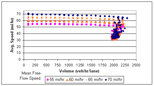
Figure 52 . Figure. Speed-volume relationship in CORSIM for a basic freeway segment.

 

The parameters altered in this step to calibrate the system performance will also affect the capacity, so care should be taken to not modify them to a degree that the capacities of key bottlenecks, as calibrated in the first step, become “uncalibrated” in this step.  Having already calibrated the capacity in the first step will likely result in the system performance MOEs of the model to be reasonably close to the field; thus, this step will likely result in fine-tuning of these parameters.  

The warning sign locations (see chapter 3 for more detail on these parameters), while coded in the base model development step (chapter 3), can have a significant impact on the system performance around on- and off-ramps.  Thus, if the above parameters do not have the desired impact in calibrating system performance, then slight modifications to the warning sign locations may be warranted.  In general, moving these warning sign locations further upstream will result in smoother, less turbulent lane changing conditions and can thus improve the system performance.

5.7.2  Calibrating Arterial System Performance

There are many parameters in CORSIM that affect the surface street system performance, so it is important to narrow the list to a few parameters that are the most sensitive to system MOEs.  A candidate list of parameters to adjust for calibrating freeway system performance includes:

• Mean discharge headway, Mean startup delay, Acceptable gap in oncoming traffic (left turns and right turns), and Cross-street acceptable gap distribution (near-side and far-side) – As described above in section 5.5, these parameters affect the capacity at surface street intersections and, as a result, also affect system performance.  Increasing these parameter values will have the effect of degrading the system performance MOEs on surface streets.  However, if these parameters were already calibrated in the bottleneck capacity step, then they should be altered here at a minimum level, if possible, to avoid undoing the capacity calibration done earlier.
• Spillback probabilities – This is a global parameter that sets probabilities for vehicles in a queue to join a downstream queue and thus block an intersection.  For closely-spaced intersections with long queues, a queue that blocks an upstream intersection will have a major impact on the system performance.  Thus, calibrating this parameter to match local conditions is important in these circumstances.
• Time to react to sudden deceleration of lead vehicle – This is a global parameter that represents the amount of time for a driver to begin decelerating after the leader begins a sudden deceleration due to perception/reaction time.  The default value is 1.0 second.  Increasing this value generally results in degraded system performance.
• Mean free-flow speed - This is a link-level parameter that represents the desired mean speed of vehicles in the absence of any impedance due to other vehicles or traffic control devices.  Each driver type has a different free-flow speed based on a global multiplier (ranges from 75 percent for conservative drivers to 127 percent for aggressive drivers).  Changing the distribution of free-flow speed by altering the global multipliers is not recommended because a recent sensitivity test showed that changing the distribution resulted in inconsistent and occasionally unrealistic impacts on system performance MOEs.⁽¹⁶⁾

As mentioned above, the mean free-flow speed should be used for system performance calibration at low levels of congestion, as the parameter is intended to model speeds at free-flow conditions.  For congested conditions, the other parameters mentioned above are better suited for calibration than free-flow speed. 

As mentioned previously, the quality of platoon progression can have a significant impact on the performance (e.g., delays, speeds, and stops) of arterials; thus, ensuring the platoon progression is realistic is an important step.  Viewing the progression of vehicles in TRAFVU can be a useful qualitative tool to verify the accuracy of the CORSIM model to the field.

The parameters altered in this step to calibrate the system performance will also affect the capacity, so care should be taken to not modify them to a degree that the capacities of key bottlenecks, as calibrated in the first step, become “uncalibrated” in this step.  Having already calibrated the capacity in the first step will likely result in the system performance MOEs of the model to be reasonably close to the field; thus, this step will likely result in fine-tuning of these parameters.

5.8 Key Decision Point: Check Overall Calibration Targets

At this point, the analyst makes a final check that all calibration targets have been satisfied.  If so, then the model is ready to proceed to the alternatives analysis step (chapter 6).  If not, then the analyst should iterate back to bottleneck capacity calibration and step through each of the three calibration steps again.  The calibration process is inherently an iterative balancing act, as altering a parameter could cause one MOE to meet its calibration target yet cause another MOE to move away from its calibration target.  This could be the case when altering a parameter for capacity calibration and then fine-tuning it later for system performance calibration, only to find that the fine-tuning caused the capacity to move outside the calibration target.  If iteration through the calibration steps is necessary, each round of iteration will likely be quicker and increasingly consist of fine-tuning parameters.

If repeated iteration of calibration still does not result in all calibration targets to be met, then the project team should review the calibration targets to make sure they are realistic given the project at hand.  The relaxing of certain calibration targets may be warranted if they do not impact critical network locations or if they will minimally impact the overall transportation decisions being made. 

If repeated iterations of calibration and the reasonable relaxation of calibration targets do not result in a satisfactory model, then the project team should reconsider the use of TSIS/CORSIM for the project at hand.  The modeled network and conditions may be beyond the capabilities of the software.  Software limitations can be identified through careful review of the software documentation.  If software limitations are a problem, then the analyst will have to work around the limitations to produce the desired performance.  If the limits are too great, the analyst might seek an alternate software program without the limitations.  Advanced analysts can also write their own software interface with TSIS/CORSIM (called a “Run Time Extension (RTE)) to overcome the limitations and produce the desired performance.  More detail on RTE functionality is provided in appendix L.

5.9 Example Problem: Model Calibration

Excelsior Boulevard and Eastbound TH 7 (nodes 127 to 145).  The calibration approach employed was consistent with that shown in Figure 45 above.

Establish Calibration MOEs and Targets

The link discharge rate just downstream of the freeway bottleneck locations was chosen as the capacity calibration MOE.  The link volumes were used as the MOE for the traffic volume calibration step.  For the system performance calibration, average link speeds and overall travel time were the primary MOEs chosen. 

An initial target was set that all model MOEs would be within 10 percent of the field measured MOEs.  Any differences beyond 10 percent would be reviewed on a case-by-case basis.

Calibrate Bottleneck Capacity 

The primary bottleneck within the study area was on northbound HWY 100 at the 25th ½ Street Exit.  The peak hour target capacity volume as measured in the field was 4,930 veh/h.  The bottleneck location extended over a larger area due to the complexity of lane drops and closely spaced ramps; however, at the end of the congestion area the discharge of traffic from the congested area was a significant traffic flow that was ideal for calibrating capacity due to the persistent upstream queues.  Figure 53 shows a schematic drawing of the northbound HWY 100 study area and existing bottleneck locations.   

The process to calibrate capacity used was to:

1. Adjust the “Car following sensitivity factor” for each driver type by a set percentage.
2. Run the model 10 times.
3. Evaluate the results.
   1. If the model capacity (measured as the discharge volume immediately downstream of the bottleneck) matches the field capacity to an acceptable level, then the capacity is considered calibrated and this step is complete.
   2. If the model capacity does not match the calibration target, then repeat the process with new “Car following sensitivity factor” values.  If altering this parameter does not result in the desired model capacity after several iterations, then other capacity-related parameters would be attempted.

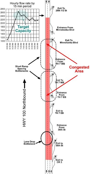
Figure 53 . Illustration. Example problem: HWY 100 freeway bottleneck locations.

The strategy used to adjust the “Car following sensitivity factors” was to systematically adjust the factor for each driver type by the same percentage.  On the first try after the base model was tested, the model capacity was found to be lower than the field measured capacity.  Thus, the “Car following sensitivity factors” were reduced by 10 percent initially to increase the capacity of the model.  During the second try, the factors were reduced by another 10 percent.  The second try did not have a significant effect on the results, so the same factors were used on the third try and, in addition, the “Pitt car following factor” was reduced from 10 to 5 to further increase the capacity of the model.  Table 13 summarizes the process used in calibrating the bottleneck capacity at the northbound HWY 100/25th ½ Street Exit.

 

Table 13 . Example problem: model adjustments for calibrating capacity.

Iteration	Car Following Sensitivity Factor for each Driver Type										Pitt Car Following Factor
	1	2	3	4	5	6	7	8	9	10
Default	1.25	1.15	1.05	0.95	0.85	0.75	0.65	0.55	0.45	0.35	10
1	1.13	1.04	0.95	0.86	0.77	0.68	0.59	0.50	0.41	0.32	10
2	1.02	0.94	0.86	0.77	0.69	0.61	0.53	0.45	0.37	0.29	10
3	1.02	0.94	0.86	0.77	0.69	0.61	0.53	0.45	0.37	0.29	5

 

Figure 54 shows the throughput volume measured in the field and with the various model iterations at the HWY 100/25th ½ Street Exit bottleneck.  As shown, the default model values resulted in the bottleneck capacity being 16.9 percent lower than that measured in the field.  However, by the third iteration, the model capacity was only 2.7 percent lower then that measured in the field, well within the 10 percent calibration target.

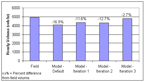
Figure 54 . Graph. Example problem: capacity calibration at northbound HWY 100/25th ½ Street Exit.

Calibrate Traffic Volumes

The HWY 100 network is linear with no alternate routes possible between each origin and destination.  Therefore, as described earlier in section 5.6, calibrating the traffic volumes was not necessary.  A check of link volumes on the HWY 100 corridor confirmed that all modeled volumes were within the 10 percent calibration target.  The link volumes are displayed in Table 14.  As shown in the table, the model volumes ranged from 3.3 percent lower to 5.5 percent higher than the field volumes.  A similar check was done for the surface streets modeled around the interchanges and also found the model volumes to be within the calibration target.

Table 14 . Example problem: NB HWY 100 AM peak traffic volumes.

Segment	Field Volume (veh/hr)	Model Volume (veh/hr)	Percent Difference
NB TH 100 – TH 62 EB Exit	3,120	3,124	+0.13
TH 62 EB Exit – TH 62 EB Entrance	2,848	2,825	-0.81
TH 62 EB Entrance – TH 62 WB Exit	3,482	3,465	-0.49
TH 62 WB Exit – TH 62 WB Entrance	2,943	2,957	+0.48
TH 62 WB Entrance – Benton Ave. Entrance	3,640	3,661	+0.58
Benton Ave. Entrance – 50th St. Exit	3,901	3,921	+0.51
50th St. Exit – 50th St. EB Entrance	3,344	3,410	+2.0
50th St. EB Entrance – 50th St. WB Entrance	3,683	3,760	+2.1
50th St. WB Entrance – Excelsior Blvd. Exit	4,021	4,103	+2.0
Excelsior Blvd. Exit – 36th St. Exit	3,044	3,140	+3.2
36th St. Exit – 36th St. Entrance	2,431	2,561	+5.4
36th St. Entrance – TH 25/TH 7 EB Exit	3,204	3,345	+4.4
TH 25/TH 7 EB Exit – TH 25/TH 7 EB Entrance	3,149	3,286	+4.4
TH 25/TH 7 EB Entrance – TH 25/TH 7 WB Exit	3,782	3,882	+2.6
TH 25/TH 7 WB Exit - TH 25/TH 7 WB Entrance	3,721	3,769	+1.3
TH 25/TH 7 WB Entrance – Minnetonka Blvd. Exit	3,963	3,964	+0.03
Minnetonka Blvd. Exit - Minnetonka Blvd. Entrance	3,913	3,879	-0.87
Minnetonka Blvd. Entrance – 25th ½ St. Exit	4,930	4,799	-2.7
25th ½ St. Exit – I-394 EB Exit	4,488	4,340	-3.3
I-394 EB Exit – Cedar Lake Rd. Entrance	2,842	2,784	-2.0
Cedar Lake Rd. Entrance – I-394 EB Entrance	3,139	3,086	-1.7
I-394 EB Entrance – I-394 WB Exit	3,590	3,527	-1.8

Note: The “model volume” represents the volumes based on the model after the capacity calibration step is complete.

Calibrate System Performance

After the model was successfully calibrated for capacity and traffic volumes, the model was calibrated for system performance.  The primary system performance measures used were average link speeds and over all travel time, while other measures such as control delay, average density, and queue lengths were used to calibrate localized congestion spots.  Several iterations of changing parameter values were tried in a similar fashion to that explained in the capacity calibration step.  The “Car following sensitivity multiplier,” “Mean free-flow speed,” and the anticipatory lane changing parameters were the main parameters used for the system performance calibration.  Table 15 shows the final calibration parameter values for the freeway system performance calibration, with those parameters changed from their default values highlighted.  In addition to those shown in the table, the anticipatory lane change parameters were adjusted just upstream of the TH 25/TH 7 EB Entrance and TH 25/TH 7 WB Entrance ramps to essentially prevent anticipatory lane changes from occurring (by changing the minimum speed trigger to 16.1 km/h (10 mi/h) and reaction point distance to 3.0 m (10 ft)).  This was done to more realistically model driver behavior in this section, as the majority of drivers were not moving to the left upstream of the merge because many of them were positioning to exit the freeway at an upcoming ramp.

Table 15 . Example problem: final system performance calibration values
for NB HWY 100.

Segment	Mean Free-flow Speed (mi/h)	Car Following Sensitivity Multiplier
NB TH 100 – TH 62 EB Exit	65	100
TH 62 EB Exit – TH 62 EB Entrance	65	100
TH 62 EB Entrance – TH 62 WB Exit	65	100
TH 62 WB Exit – TH 62 WB Entrance	65	100
TH 62 WB Entrance – Benton Ave. Entrance	65	100
Benton Ave. Entrance – 50th St. Exit	65	100
50th St. Exit – 50th St. EB Entrance	65	100
50th St. EB Entrance – 50th St. WB Entrance	65	100
50th St. WB Entrance – Excelsior Blvd. Exit	65	120
Excelsior Blvd. Exit – 36th St. Exit	65	140
36th St. Exit – 36th St. Entrance	65	140
36th St. Entrance – TH 25/TH 7 EB Exit	60	120
TH 25/TH 7 EB Exit – TH 25/TH 7 EB Entrance	60	120
TH 25/TH 7 EB Entrance – TH 25/TH 7 WB Exit	60	120
TH 25/TH 7 WB Exit - TH 25/TH 7 WB Entrance	60	110
TH 25/TH 7 WB Entrance – Minnetonka Blvd. Exit	60	100
Minnetonka Blvd. Exit - Minnetonka Blvd. Entrance	60	90
Minnetonka Blvd. Entrance – 25th ½ St. Exit	60	80
25th ½ St. Exit – I-394 EB Exit	65	90
I-394 EB Exit – Cedar Lake Rd. Entrance	65	100
Cedar Lake Rd. Entrance – I-394 EB Entrance	65	100
I-394 EB Entrance – I-394 WB Exit	65	100

Note: Shaded cells represent values that were changed from their default during the calibration process.

As a result of the calibration efforts, the average speeds of all links were within six percent of the field speeds during the AM peak hour and within five percent during the PM peak hour for northbound HWY 100.  A few individual links were more than 10 percent away from the field measurements, but these were considered acceptable given the difficulty in matching speeds for a large freeway section with congested conditions.  Figure 55 shows the results of the AM peak hour average speed calibration for northbound HWY 100.  As shown, the model replicates the speeds on northbound HWY 100 much more closely after calibration than with the base model. 

Figure 55 . Graph. Example problem: speed calibration results for
northbound HWY 100 during AM peak.

While the graph above shows a calibration that was performed using aggregated one-hour average speeds, the variations in 15-minute average speeds over the entire three-hour analysis period were also calibrated at key locations.  Figure 56 shows a typical graph that was used to compare the field and model speeds on individual links.  As shown, the model slightly underestimates the field speeds but matches the general speed profile as it decreases over time.

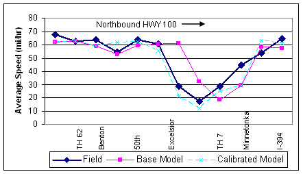
Figure 56 . Graph. Example problem: speed calibration results for
northbound HWY 100 at WB TH 7 Exit during AM peak.

A similar calibration process was used to calibrate other system performance MOEs, such as overall travel time through the corridor, density and queuing at congested locations, and control delay and queuing at the signalized intersections at the interchange terminals.

Key Decision Point: Check Overall Calibration Targets

A review was completed of all calibration MOEs and whether they met the established calibration targets.  The MOEs were found to be well-calibrated and, while a few MOEs such as average link speeds exceeded the target, the model overall represented the field conditions as well as could be expected given that this is a large simulation model with existing congestion.

After discussing the calibration results with the project team, consensus was established that the model was fully calibrated and ready to proceed to the alternatives analysis step.