6.0 Alternatives Analysis
Project alternatives analysis is the sixth step in the CORSIM analysis process. It is often the primary reason for developing and calibrating the model. The lengthy model development process has been completed and now itis time to put the model to work. (7)
The analysis of project alternatives involves the forecasting of the future demand for the base model and the testing of various project alternatives against this baseline future demand. The analyst must run the model several times, review the output, extract relevant statistics, correct for biases in the reported results, and perform various analyses of the results. These analyses may include hypothesistesting, computation of confidence intervals, and sensitivity analyses to further support the conclusions of the analysis.
The alternatives analysis task consists of several steps:
- Development of Baseline Demand Forecasts.
- Generation of Project Alternatives for Analysis.
- Selection of Measures of Effectiveness (MOEs).
- Application of CORSIM Model (Runs).
- Tabulation of Results.
- Evaluation of Alternatives.
Documenting the development of the alternative networks and analysis of the alternatives is very important to the success of the study and it makes the final documentation much easier to understand. Decisions, procedures, and assumptions made during the alternative analysis process should be documented so that when the study is reviewed in the future it is clear why the study was done as it was. For example, traffic forecasts need to be part of the alternatives analysis of a future year’s traffic; however, traffic forecasts may be different for different alternatives due to changes in traffic routing and circulation patterns. The results of an analysis may be summarized in a summary report that contains the MOEs for the alternatives tested. Such a summary report could then be later incorporated into the final documentation.
6.1 Baseline Demand Forecast
This step consists of establishing the future level of demand to be used as a basis for evaluating project alternatives. Additional information and background regarding the development of traffic data for use in highway planning and design may be found in National Cooperative Highway Research Program (NCHRP) Report 255, Highway Traffic Data for Urbanized Area Project Planning and Design.
6.1.1 Demand Forecasting
A significant component to the analysis of alternatives is the development of traffic forecasts. This process is quite involved and relies on estimates and assumptions to determine what the traffic volumes will be in the future.(2) Forecasting techniques include:
- Regional Travel Demand Models. The regional models are large-scale models that assign traffic to the roadway system based on desired travel between areas called Traffic Analysis Zones (TAZs) and major roadways that leave the study areas. Within each TAZ, trips are estimated based on the socio-economic information including residential population and employment. Trips are assigned to the roadway network based on the desired destination between zones and the relative congestion on each road. The regional forecast model will take into account parallel routes and divert traffic accordingly. The results from travel demand models require careful review, as the estimates of capacity are at a planning level and may not take into account detailed operational constraints, such as queue blockages or freeway weaving areas.
- Applying Historical Growth Patterns. The analyst may seek to develop demand forecasts based on historic growth rates. A trend-line forecast might be made, assuming that the recent percentage of growth in traffic will continue in the future. These trend-line forecasts are most reliable for relatively short periods of time (5 years or less). They do not take into account the potential of future capacity constraints to restrict the growth of future demand. Strong caution must be used when historical growth is applied; a mature corridor may not grow at a high rate or the growth rate may not take into account realistic system capacities and possible diversions to other routes.
- ITE Trip Generation Methods. The Institute of Transportation Engineers maintains a Trip Generation Manual,(17) which contains trip rates for different land use types and sizes. This methodology would involve adding traffic to existing traffic counts based on new development. This method would not take into account background growth outside of the study area.
- Hybrid of all the above. It is possible to employ all of these methods to develop traffic forecasts.
As discussed earlier in section 3.3, entering traffic demand in CORSIM using 15-minute time periods throughout the entire peak period (i.e., the onset of congestion through the dissipation of congestion) should adequately represent the dynamic nature of demand in a study area. However, forecasting the traffic demand for a future year is not a precise science. While estimating daily traffic and peak hour traffic for a future year is difficult, estimating the future year demand in 15-minute increments is even more difficult.
In order to analyze peak periods in CORSIM for the future condition, the analyst could first forecast the future year peak hour demand based on the forecasting techniques discussed above and then factor the existing 15-minute demands uniformly by the future peak hour demand divided by the existing peak hour volume. This is similar to applying a peak hour factor in the HCM. In essence, the existing peak period traffic pattern is applied to the future in order to analyze the build-up, duration, and dissipation of congestion.
6.1.2 Constraining Demand to Capacity
Regardless of which method is used to estimate future demand, care must be taken to ensure that the forecasts are a reasonable estimate of the actual amount of traffic that can arrive within the analytical period at the study area. Regional model forecasts are usually not well constrained to system capacity and trend-line forecasts are totally unconstrained. Appendix F of Volume III provides a method for constraining future demands to the physical ability of the transportation system to deliver the traffic to the model study area.(7)
6.1.3 Allowance for Uncertainty in Demand Forecasts
All forecasts are subject to uncertainty. It is risky to design a road facility to a precise future condition given the uncertainties in the forecasts. There are uncertainties in both the probable growth in demand and the available capacity that might be present in the future. Slight changes in the timing or design of planned or proposed capacity improvements outside of the study area can significantly change the amount of traffic delivered to the study area during the analytical period. Changes in future vehicle mix and peaking can easily affect capacity by 10 percent. Similarly, changes in economic development and public agency approvals of new development can significantly change the amount of future demand.(7) Thus, it is good practice to explicitly plan for a certain amount of uncertainty in the analysis. This level of uncertainty is the purpose of sensitivity testing (explained further in section 6.6).
6.2 Generation of Project Alternatives
In this step, the analyst generates improvement alternatives based on direction from the decision makers and through project meetings. They will probably reflect operational strategies and/or geometric improvements to address the problems identified based on the baseline demand forecasts. The generation of alternatives should consider at the minimum:
- Performing CORSIM analyses of the baseline demand forecasts (“future no-build” alternative) to identify deficiencies in the transportation system or performance goals and objectives which the “build” alternative(s) will support. The future analysis years could consist of interim and opening years of the improvement(s) considered and future design year established in the scoping phase of the project (refer to section 1.2 for more detail).
- Performing CORSIM analyses of potential improvements (“future build” alternatives) that solve one or more of the identified problems in the baseline alternatives. In addition to considering traditional infrastructureand geometric improvements, alternatives should also consider transportation system management strategies (e.g., ramp metering, traffic signal coordination, and improved traveler information) as well as alternative transportation mode strategies (e.g., HOV lanes and ramps and improved transit service).
One difficulty in generating alternatives is maintaining control of the alternatives and the base network. The analyst must make sure the base network is used as the basis for all alternatives. Invariably, after all the base model development and error checking is done and alternatives have been developed, an error will be found in the base model that affects all of the alternatives. Making the change in the base model and all of the alternatives can be tedious and error prone. Therefore, using an automated way to make changes is beneficial.
The TRF Manipulator tool can be used in a script to repeatedly open a CORSIM (*.TRF) input file, manipulate the contents, and save the file with a new name. Well written scripts can make this tool do much of the previously intensive and error prone task of changing data. A change file specific to the changes for each alternative can be applied to the base network making the creation of alternative network files quite simple and repeatable. The TRF Manipulator tool uses the TRF format database to know what columns of text on the specified record entries to manipulate. The TRF Manipulator is also very useful when performing sensitivity studies. It can be used in a nested loop to set a parameter then increment it multiple times. This tool has many functions to change different types of data. For more information refer to the TSIS Script Tool User’s Guide.(6)
6.3 Selection of Measures of Effectiveness (MOEs)
MOEs are the system performance statistics that best characterize the degree to which a particular alternative meets the project objectives (which were determined in the Project Scope task). Thus, the appropriate MOEs are determined by the project objectives and agency performance standards rather than what is produced by the model. The selection of appropriate MOEs ideally would have been developed through the consensus of all stakeholders at the beginning of the project (Project Scope task) concurrently with the development of the project objectives; however, if this was not the case, then MOEs should be selected at this point so that the analyst understands which MOEs to base his/her findings upon.
The following project objectives were given in chapter 1 as an example of establishing objectives that are specific and measurable (note that these represent only an example):
- Provide for minimum average freeway speeds of 75 km/h (47 mi/h) throughout the peak period between Points A and B.
- Provide for ramp operations which do not generate queues or spillback which impact operations on the freeway or major crossroad.
- Arterial operations within 4.0 km (2.5 mi) of freeway interchanges maintain an average speed of 55 km/h (34 mi/h) and arterial intersections do not result in phase failure or queue spillback into adjacent intersections.
In this example, the MOEs reported for each alternative would thus need to reflect measurement of average speeds on the freeway, queues on the ramps, average speeds on the arterial, queues on the arterial approaches, and phase failure at the arterial intersections.
Because the selection of appropriate MOEs depends on the project objectives, needs and priorities of the stakeholders, agency performance standards, and/or past practice in the region, this section does not recommend specific MOEs to select; rather, this section highlights possible candidate MOEs typically produced by CORSIM so that the analyst can appreciate what output might be available for constructing the desired MOEs. CORSIM calculates hundreds of possible MOEs, thus it is important that the key MOEs for the particular study be selected upfront before the analyst begins the alternatives analysis.
An understanding of how MOEs are defined and accumulated in CORSIM is critical when evaluating the performance of alternatives. For example, understanding how and when to report cumulative, time period-specific, or time interval-specific MOEs is important when identifying and evaluating location-specific problem areas. Appendix H (Understanding CORSIM Output) contains more detailed information on understanding and interpreting CORSIM MOEs.
6.3.1 Candidate MOEs for Overall System Performance
Many MOEs of overall system performance can be computed directly or indirectly from the following three basic system performance measures as reported in the TSIS Output Processor. (Note: This is the terminology used in CORSIM):
- Travel Distance Total (Vehicle-miles traveled (VMT)).
- Travel Time Total (Vehicle-hours traveled (VHT)).
- Speed Average.
These three basic performance measures can also be supplemented with other model output, depending on the objectives of the analysis. For example, Delay Travel Total is a useful overall system performance measure for comparing the congestion-relieving effectiveness of various alternatives. The number of stops is a useful indicator for traffic signal coordination studies. Another indicator is the time to onset of a congested state, such as speed below 88.5 km/h (55 mi/h) or a signal phase failure (i.e., a vehicle queue at a traffic signal does not clear the intersection in a single green phase). These indicators provide insight that one alternative may remain in a desired operational state until a specific point in time, while another alternative may remain in a desired operational state for a shorter or longer period of time.
In order to understand the characteristics of each alternative, multiple system-wide MOEs should be looked at and considered. The Traffic Analysis Toolbox, Volume VI: Definition, Interpretation, and Calculation of Traffic Analysis Tools Measures of Effectiveness recommends that a “starting set” of basic MOEs first be evaluated: throughput, mean delay, travel time index, freeway segments at breakdown, and surface street intersections with long queues, turn bay overflows, and exit blockages.(18) These basic MOEs are analogous to the initial exams given to every patient checking into the emergency room (i.e., temperature, pulse, blood pressure, and blood oxygen), which give the doctors a basic understanding of the general health of the patient and some indication of fields to investigate for the source of the problem. Similarly, the basic MOEs serve as this initial high-level screening of the overall performance of the system. Then, based on these basic MOEs, a more detailed analysis of specific MOEs at hotspot locations can be used to further understand the extent and nature of the problems.(18)
Many CORSIM studies cover large areas with multiple hours to properly capture the spatial and temporal extent of congestion. While reporting the average of a particular MOE for the entire study area and analysis period will help prioritize the overall effectiveness of an alternative, a more insightful approach is to report the selected MOEs by segment or section of roadway and by time period (i.e., 15-minute period). Reporting the MOEs by spatial bounds and temporal periods will allow the extent and location of congestion to become evident for each alternative. Comparing the MOE results between alternatives is discussed further in section 6.6.
6.3.2 Candidate MOEs for Localized Problems
In addition to evaluating overall system performance, the analyst should also evaluate if and where there are localized system breakdowns (“hot spots”). Hot spot locations can often initially be identified by reviewing the CORSIM animation; however, care should be taken in relying on the animation of a single CORSIM run to identify hot spots (discussed further in section 6.6). While reviewing the animation can be a powerful tool in identifying localized problems, link-level MOEs from CORSIM output should be evaluated over multiple runs to quantify the location, severity, and extent of hot spots. Several MOEs that can be used to identify these breakdowns or hot spots include:
- Persistent queue that lasts too long. There is no single CORSIM MOE that reports the extent and duration of a queue that spans multiple links. On freeways (reported in the FRESIM output), the location and extent of queues can be estimated based on low average speeds or high average densities for consecutive links. Queuing can also be identified if a vehicle back-up warning message is generated (e.g., “Warning – 100 Vehicles Backed Up Behind Node 8001”), which occurs when queues on the network prevent vehicles from entering the network at an entry node. This warning message can be viewed while CORSIM is running and is also reported in the output file (*.OUT file). On surface streets (reported in the NETSIM output), long queues can be identified based on the “Average Queue Length by Lane” or “Maximum Queue Length by Lane” MOEs, which are generated for each link. Queuing can also be estimated based on high delay values on specific links (e.g., “Queue Delay per Vehicle”).
- A signal phase failure (a vehicle queue at a traffic signal does not clear the intersection in a single green phase). CORSIM output includes a “Phase Failure” MOE for each surface street link, which is a cumulative count of the number of times during the simulation that the queue at a signal fails to be discharged completely during a green phase.
- A blocked link or a queue that spills back onto an upstream intersection. CORSIM output includes warning messages when surface street links experience queue spillback (i.e., queues extend to an upstream link). The warning message states when spillback begins and ends, which could occur multiple times throughout the duration of a simulation run.
- Freeway merging or weaving area that creates a bottleneck condition resulting in upstream queues and congestion. As stated above, the location and extent of queuing due to a freeway bottleneck can be estimated based on low average speeds or high average densities for consecutive links.
6.3.3 Choice of Average or Worst Case MOEs
The analyst needs to determine if the alternatives should be evaluated based on their average predicted performance or their worst case predicted performance. As discussed in Chapter 5, accumulating and reporting statistics over many runs is easily done with the TSIS tools. The standard deviation of the results can be computed and used to determine the confidence interval for the results.
The worst case result for each alternative is slightly more difficult to compute. It might be tempting to select the worst case result from the simulation model runs; however, the difficulty is that the analyst has no assurance that if the model were to be run a few more times, an even worse result might be computed. Thus, the analyst never knows if they have truly obtained the worst case result. The solution is to compute the 95th percentile probable worst outcome based on the mean outcome and an assumed normal distribution for the results.(7) The equation below can be used to make this estimate:
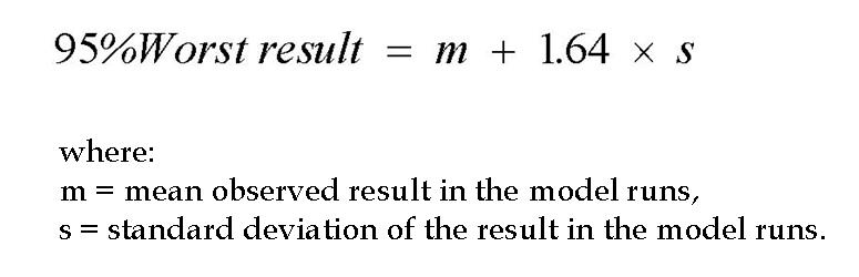
Figure 57. Equation. Calculating the 95th percentile probable worst outcome.
6.4 Model Application
The calibrated CORSIM model is applied, or ran, in this step to compute the MOEs for each alternative. The CORSIM User’s Guide(1) describes in detail the steps required to run CORSIM. The purpose of this section, however, is to discuss some key issues that the analyst should consider when running CORSIM for the alternatives analysis.
6.4.1 Multiple CORSIM Runs
Due to the stochastic nature of CORSIM, the results from individual runs can vary significantly, especially for facilities operating at or near capacity. Thus, it is necessary to run CORSIM multiple times with different random number seeds to gain an accurate reflection of the performance of the alternatives. The CORSIM Driver Tool has a built-in multiple-run capability and a built-in output processor that collects statistics from each run and summarizes them.
The multi-run capability runs a test case multiple times, changing the random number seeds for each run. Thus, by default CORSIM will change the random seed values for multiple runs of the same CORSIM file (using the “random.rns” file). When running a separate CORSIM file (i.e., different alternative) multiple times, the output processor will subsequently use the same set of random seed values in the “random.rns” file. Using the same set of random seed values among all alternatives will ensure that the only difference in output among alternatives is due to the differences in the alternatives themselves (i.e., different traffic demands, geometries, traffic control strategies, etc.).
Overall, using the multi-run function in the output processor will automatically change the random seed values for multiple runs of the same CORSIM file and use the same set of random seed values across multiple alternatives. The output processor does allow an analyst to change the default set of random seed values if necessary. Refer to Appendix D for more information on the usage of random seed values in CORSIM.
Section 5.4 discusses in more detail how to calculate the appropriate number of runs for each alternative. Also, the CORSIM User’s Guide(1) contains detailed information on setting up and performing multiple simulation runs in CORSIM.
6.4.2 Exclusion of Initialization Period
The artificial period where the simulation model begins with zero vehicles on the network (referred to as the “initialization period” or “fill period”) must be excluded from the reported statistics for system performance. CORSIM will do this automatically. The initialization period typically ends when equilibrium has been achieved. Equilibrium is achieved when the number of vehicles entering the system is approximately equal to the number leaving the system. The algorithm used by CORSIM does not work properly in all circumstances. For example, if the data collected during a run shows a sharp decrease in value soon after the initialization period, it is a good indication that equilibrium was not reached. Thus, the analyst should check the CORSIM output file (*.OUT file) to ensure equilibrium has been reached in the CORSIM run. Model output should not be used if equilibrium has not been reached, as the results will not represent the actual volumes attempted to be modeled. Appendix C has a more detailed discussion of the initialization period.
6.4.3 Impact of Alternatives on Demand
The analyst should consider the potential impact of alternative improvements on the base model forecast demand. This should take into consideration the effects of a geometric alternative and/or a traffic management strategy. The analyst should then make a reasonable effort to incorporate any significant demand effects into the analysis.
For example, if improvements are added to serve the existing 4,000 vehicles per hour, the improvements themselves may draw, or induce, an additional 500 vehicles per hour after the improvements are completed. Drivers may alter their route to take advantage of the improvements and create an unforecasted demand change. For a second example, if a freeway interchange is inserted between two existing interchanges, the exit and turn percentages at the existing interchanges will most likely change from the base model percentages. New turning fractions must be estimated by repeating the traffic assignment based on the improvements.
6.4.4 Signal/Meter Control Optimization
CORSIM does not optimize signal timing or ramp meter controls. Thus, if the analyst is testing various demand patterns or alternatives that significantly change the traffic flows on specific signalized streets or metered ramps, he or she may need to include a signal and meter control optimization step within the analysis of each alternative. This optimization might be performed offline using a macroscopic signal timing or ramp metering optimization model. Or, the analyst may run CORSIM multiple times with different signal settings and manually seek the signal setting that gives the best performance. Refer to the Signal Optimization discussion in section 3.4 for information on third party products that can be used to aid in developing optimized signal timing settings.
6.5 Tabulation of Results
The process of collecting and summarizing CORSIM output using the output processor is discussed briefly in section 5.4 and in more detail in the CORSIM User’s Guide(1). Tabulating the results for the alternative analysis in this chapter is essentially the same process as used in chapter 5 with possible exceptions of selecting different MOEs and running various future-year alternatives.
6.5.1 Numerical Output
TSIS and CORSIM report the numerical results of the model run in text output files or spreadsheet files. The results are summarized over time and/or space. It is critical that the analyst understands how CORSIM has accumulated and summarized the results to avoid pitfalls in interpreting the numerical output.
The CORSIM output file (*.OUT file) accumulates the data over time intervals and either reports the cumulative sum, the maximum, or the cumulative average. The output processor can also report the data specific to the time interval or time period. Interval-specific data can be useful for comparing volume data that varies over time periods or for measuring the extent and duration of queuing and congestion dynamically over time through the entire simulation. Changes in the performance of the network are reflected immediately when using interval-specific data, whereas cumulative data, which is averaged over the duration of the entire run, takes a long time to reveal the changes.
CORSIM can report the results for specific points on a link in the network by using detectors or data stations or for aggregated data over the entire link. The point-specific output is similar to what would be reported by detectors in the field. Link-specific values of road performance are accumulated over the length of the link and, therefore, will vary from the point data. CORSIM also reports results for network wide or subnetwork wide, bus station or bus route, vehicle fleet, or link aggregation statistics. Appendix H has a summary of all MOEs available through the output processor.
6.5.2 Correcting Biases in the Results
The geographic and temporal model limits should be sufficient to include all congestion related to the base case and all of the alternatives. An example of this would be modeling a network where an entry node has spillback. Otherwise, the model will not measure all of the congestion associated with an alternative, thus causing the analyst to underreport the benefits of an alternative.
To make a reliable comparison of the alternatives, it is important that vehicle congestion for each alternative be accurately tabulated by the model. This means that congestion (vehicle queues and/or low travel speeds) should not extend physically or temporally beyond the geographic or temporal boundaries of the simulation model. Congestion that overflows the geographic limits of the network will be reported by CORSIM, both on the screen at run time and in the output (*.OUT) file.
Ideally, the simulation results for each alternative would have the following characteristics:
- All of the congestion begins and ends within the simulation study area.
- No congestion starts before or ends after the simulation period.
- No vehicles are unable to enter the network from any entry point during any time step of the simulation.
It may not always be feasible to achieve all three of these conditions, so it may be necessary to make adjustments for congestion that is missing from the model output. Some possible adjustments are described below.
Adjustment of Output for Blocked Vehicles
If simulation alternatives are severely congested, then CORSIM may be unable to load vehicles onto the network. Some may be blocked from entering the network on the periphery. Some may be blocked from being generated on internal links. These blocked vehicles will not be included in the travel time or delay statistics for the model run. The best solution is to extend the network back to include the maximum back of the queue. If this is not feasible, then the analyst should correct the reported delay to account for the unreported delay for the blocked vehicles.
CORSIM will tally the excess queue that backs up outside the network as “blocked” vehicles (vehicles unable to enter the network). The MOEs collected at the entry links provide the number of vehicles that were delayed, the total time vehicles were delayed, and the average delay per vehicle. When a block of fifty vehicles back up at an entry point, there is a message displayed to the screen and written to the output (*.OUT) file (e.g., “Warning – 100 Vehicles Backed Up Behind Node 8001”). The delay resulting from blocked vehicles should then be added to the model-reported delay for each model run.
Adjustment of Output for Congestion Extending Beyond the End of the Simulation Period
Vehicle queues that are present at the end of the simulation period may affect the accumulation of total delay and distort the comparison of alternatives (cyclical queues at signals can be neglected). The “build” alternative may not look significantly better than the “no-build” alternative if the simulation period is not long enough to capture all of the benefits. The best solution is to extend the simulation period until all of the congestion that built up over the simulation period is served. If this is not feasible, the analyst can make a rough estimate of the residual delay that was not captured by using the method outlined in section 6.5.3 of Volume III.(7)
6.6 Evaluation of Alternatives
The evaluation of alternatives using CORSIM output involves the interpretation of system performance results and the assessment of the robustness of the results. Methodologies for the ranking of alternatives and cost-effectiveness analyses are well documented in other reports and are not discussed here.
6.6.1 Interpretation of System Performance Results
This subsection explains how to interpret the differences between alternatives for three basic system performance measures (Travel Distance Total, Travel Time Total, and Average Speed) (as reported by the Output Processor).
Travel Distance Total (Vehicle-Miles Traveled)
Travel Distance Total provides an indication of total travel demand (in terms of both the number of trips and the length of the trips) for the system. Travel Distance is computed as the product of the number of vehicles traversing a link and the length of the link, summed over all links. Increases in Travel Distance generally indicate increased demand. Since Travel Distance is computed as a combination of the number of vehicles on the system and their length of travel, it can be influenced both by changes in the number of vehicles and changes in the trip lengths during the simulation period. The following can cause changes in Travel Distance between one alternative and the next:
- Random variations between one alternative and the next. Increasing the number of runs for each alternative will reduce the difference in average Travel Distance due to random variations in traffic. Thus, any differences observed will only be due to the differences in the alternatives.
- Changed demand.
- Increased congestion may also reduce the number of vehicles that can complete their trip during the simulation period, also decreasing Travel Distance.
- Inability of the model to load the coded demand onto the network within the simulation period. Increased congestion may force the model to store some of the vehicle demand outside the network due to bottlenecks at loading points; in this situation, increased congestion may actually lower Travel Distance because the stored vehicles do not travel any distance during the simulation period.(7)
- Changed capacity. Increasing the capacity from one alternative to the next (e.g., from base case to a build alternative) can increase the number of vehicles served and thus produce a higher Travel Distance Total for an alternative that improves the system.
Travel Time Total (Vehicle-Hours Traveled)
Travel Time Total provides an estimate of the amount of time expended traveling on the system. Decreases in Travel Time generally indicate improved system performance and reduced traveling costs for the public. Travel Time is accumulated every second a vehicle is on the link. The Travel Time for all links is summed to get the system Travel Time. Travel Time can be influenced by both changes in demand (the number of vehicles) and changes in congestion (travel time). Changes in Travel Time between one alternative and the next can be caused by the following:
- Random variations between one alternative and the next.
- Changed demand.
- Changed congestion.
- Demand stored off-network because of excessive congestion at load points. Increased congestion that causes demand to be stored off-network may reduce Travel Time if the software does not accumulate delay for vehicles stored off-network.(7)
- Changed capacity. Increasing the capacity from one alternative to the next (e.g., from base case to a build alternative) can increase the number of vehicles served and thus produce a higher Travel Time Total for an alternative that improves the system.
Speed Average
Speed Average is an indicator of overall system performance. Higher speeds generally indicate reduced travel costs for the public. The mean system speed is computed as Travel Distance Total divided by Travel Time Total. Changes in the average speed between one alternative and the next can be caused by the following:
- Random variations between one alternative and the next.
- Changed link speeds and delays caused by congestion.
- Changes in vehicle demand.
- Changes in the number of vehicles stored off-network caused by excessive congestion at loading points.(7)
Delay Travel Total
Delay Travel Total is useful because it reports the portion of total travel time that is most irritating to the traveling public. CORSIM defines Delay Travel Total as the Travel Time Total minus the Move Time Total where Move Time Total is the theoretical travel time for all vehicles if they were moving at the free-flow speed, calculated as the link travel distance total divided by the free-flow speed, computed by link and summed for all links in the network. Changes in the total delay time between one alternative and the next can be caused by the following:
- Random variations between one alternative and the next.
- Changed delays caused by congestion.
- Changes in vehicle demand.
- Changes in signal timing.
- Changes in the number of vehicles stored off-network caused by excessive congestion at loading points.
Travel Time Studies
Travel time studies are beneficial to understanding the benefits of various build alternatives. They provide context to the public. Using probe vehicles to travel through the network along common commutes provides a connection for the public and decision makers. Average travel times on common routes can also be estimated by aggregating the average travel times of all links in particular routes of interest.
6.6.2 Hypothesis Testing
When CORSIM is run several times for each alternative, the analyst may find that the variance in the results for each alternative is close to the difference in the mean results for each alternative. The analyst needs to determine if the differences in the alternatives are statistically significant. The analyst also should determine to a certain degree of confidence that the observed differences in the simulation results may be caused by the differences in the alternatives and not just the result of using different random number seeds or of insufficient runs. This is the purpose of statistical hypothesis testing. Hypothesis testing determines if the analyst has performed an adequate number of repetitions for each alternative to truly tell the alternatives apart at the analyst’s desired level of confidence. Hypothesis testing is discussed in more detail in Appendix E of Volume III.(7)
6.6.3 Confidence Intervals and Sensitivity Analysis
Confidence intervals are a means of recognizing the inherent variation in stochastic model results and conveying them to the decision maker in a manner that clearly indicates the reliability of the results. For example, a confidence interval would state that the mean delay for alternative “X” lies between 35.6 sec and 43.2 sec, with a 95-percent level of confidence. If the 95-percent confidence interval for alternative “Y” overlaps that of “X”, then the analyst may not be able to decisively state that one alternative is statistically different than the other. The analyst would need to perform hypothesis testing as discussed above. Computation of the confidence interval is explained in more detail in Appendix B of Volume III.(7)
A sensitivity analysis is a targeted assessment of the reliability of the simulation results, given the uncertainty in the input values or assumptions. The analyst identifies certain input values or assumptions about which there is some uncertainty and varies them to see what their impact might be on the CORSIM results. Additional model runs are made with changes in demand levels and key parameters to determine the robustness of the conclusions from the alternatives analysis. The analyst may vary the following parameters to determine how sensitive the model is to change:
- Demand.
- Street improvements assumed to be in place outside of the study area.
- Parameters for which the analyst has little information.
A sensitivity analysis of different demand levels is particularly valuable when evaluating future conditions. Demand forecasts are generally less precise than the ability of CORSIM to predict their impact on traffic operations. A 10-percent change in demand can cause a facility to shift from operating at 95 percent of capacity to 105 percent of capacity, resulting in an exponential increase in the predicted delay and queuing for the facility.
The analyst should estimate the confidence interval for the demand forecasts and test CORSIM at the high end of the confidence interval to determine if the alternative still operates satisfactorily at the potentially higher demand levels.
The analyst should plan for some selected percentage above and below the forecasted demand to allow for these uncertainties in future conditions. The analyst might consider at least a 10-percent margin of safety for the future demand forecasts. A larger range might be considered if the analyst has evidence to support the likelihood of greater variances in the forecasts. To protect against the possibility of both underestimates and overestimates in the forecasts, the analyst might perform two sensitivity tests—one with 110 percent of the initial demand forecasts and the other with 90 percent of the initial demand forecasts—for establishing a confidence interval for probable future conditions.
Street improvements assumed to be in place outside the simulation study area can also have a major impact on the simulation results by changing the amount of traffic that can enter or exit the facilities in the study area. Sensitivity testing would change the assumed future level of demand entering the study area and the assumed capacity of facilities leaving the study area to determine the impact of changes in the assumed street improvements.
The analyst may also run sensitivity tests to determine the effects of various assumptions about the parameter values used in the simulation. If the vehicle mix was estimated, variations in the percentage of trucks might be tested. The analyst might also test the effects of different percentages of familiar drivers in the network.
6.6.4 Comparing Results to Other Traffic Analysis Tools
Analysts may attempt to compare the results of CORSIM to the results from other traffic analysis tools. The reasoning for this comparison varies. These types of comparisons however are not recommended because of the differences in how each traffic analysis tool defines and calculates the respective MOEs.
Each tool (including the Highway Capacity Manual (HCM) method) has notably different definitions of what constitutes stopped and queued vehicles and because the tools also vary significantly in the determination of which vehicles to include in the computations of MOEs. For example, some simulation tools compute the vehicle-miles traveled only for vehicles that enter the link during the analysis period, others include the vehicles present on the link at the start of the period and assume that they travel the full length of the link, and yet others include only the vehicles able to exit the link during the analysis period (CORSIM included).(18)
Further, simulation models (including CORSIM) are not directly translatable into HCM level of service (LOS) measures because the HCM bases hourly level of service on the performance of the facility during the peak 15-consecutive-minute period within the analysis hour. Also, most simulation models (including CORSIM) report the density of vehicles, while the density used in HCM LOS calculations for uninterrupted flow facilities is the passenger-care equivalent in passenger car units (pcu) of the actual density of vehicles on the facility.(18)
As a result, it is not feasible for an analyst to take the macroscopic output from one tool, apply a conversion factor (or procedure) and compare the results to that of another tool. This means that looking up HCM LOS using MOEs produced by CORSIM is prone to bias and error and is thus not appropriate.(18)
For similar reasons, analysts should not be switching tools in the middle of a comparison between alternatives. One set of tools should be consistently used to evaluate MOEs across all alternatives. One should not evaluate one alternative with one tool, another alternative with a second tool, and then use the MOEs produced by both tools to select among the alternatives. Comparison of results between tools is possible only if the analyst looks at the lowest common denominator shared by all field data collection and analytical tools: vehicle trajectories. Further discussion on this topic is provided in Volume VI.(18)
6.6.5 Reviewing Animation Output
Animation is a very powerful tool to convey differences in alternatives. However, one problem with animating an alternative is selecting which individual case to animate. If the stochastic processes are set up correctly, each run is a valid representation. However, it is not possible to animate the mean values of all MOEs, so the analyst must choose an individual run (defined by a set of random number seeds) that demonstrates a representative run of the MOEs of interest. The analyst must determine if they want to animate the worst case, best case, or mean case. One technique to select a representative mean case is to calculate the nearest neighbor value, as discussed below.
Nearest Neighbor
The CORSIM output processor can calculate the “nearest neighbor” value for each simulation run. The nearest neighbor value is the sum of the absolute values of the difference between the sample value at each interval and the sample mean for that interval. The formula to compute the nearest neighbor value for “run j” is:

Figure 58. Formula. Determining the nearest neighbor value.
The simulation run with the lowest nearest neighbor value can be thought of as the run that most closely matches the mean throughout the duration of the simulation. This is useful if an analyst wants to generate animation files that are representative of the average results.
Figure 59 shows the results of an example simulation case with four different runs, along with the mean over all four runs. A single MOE was selected, and the mean value of the MOE for each of the ten time intervals is plotted on the graph. As the figure indicates, all four runs have the same overall mean value of five when averaging over all ten time intervals. Locating the mean of each interval in the graph, runs A and D have nearest neighbor values of 22, while run B has a nearest neighbor value of 17. Run C has a nearest neighbor value of eight and, as can be seen graphically, is nearest to the mean of the interval value.
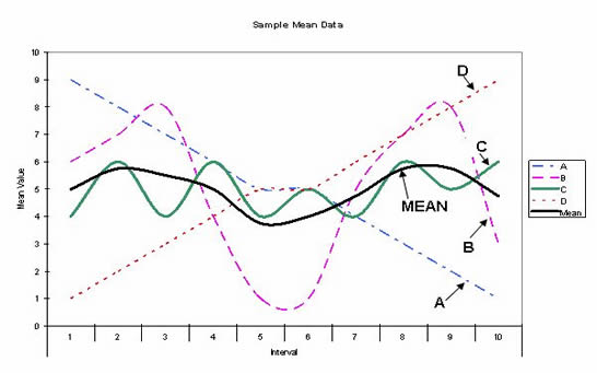
Figure 59 . Graph. Sample mean data graph for nearest neighbor example.
The example and graph above shows the nearest neighbor for a specific MOE. Each MOE may have different runs that are the nearest neighbor. Selecting the run that best represents the mean values requires determining what MOEs are most important or which run is consistently close to being the nearest neighbor. In order to use Travel Distance Total, Travel Time Total, and Average Speed, the run that is consistently the lowest should be chosen. It most likely will not be the lowest for all MOEs. Table 16 shows an example of nearest neighbor data for 10 runs of a test case. The sum of the nearest neighbor values shows that run nine is the run that most closely matches the mean for all three MOEs.
Table 16 . Example nearest neighbor calculation with multiple MOEs.
Run |
Nearest Neighbor Value |
|||
|---|---|---|---|---|
Travel Time Total |
Travel Distance |
Average Speed (mi/h) |
Sum |
|
1 |
5.8 |
113.4 |
9.7 |
128.9 |
2 |
8.6 |
125.0 |
15.8 |
149.4 |
3 |
5.3 |
96.4 |
11.7 |
113.4 |
4 |
5.6 |
107.9 |
10.7 |
124.2 |
5 |
5.9 |
94.8 |
9.8 |
110.5 |
6 |
7.8 |
118.3 |
15.6 |
141.7 |
7 |
10.8 |
113.6 |
20.6 |
145 |
8 |
8.9 |
120.9 |
17.9 |
147.7 |
9 |
6.0 |
82.0 |
9.9 |
97.9 |
10 |
6.1 |
143.4 |
9.2 |
158.7 |
Note: Shaded cells represent the lowest nearest neighbor values for each column.
The pitfall of using a global summary statistic (such as VHT) to select a model run for animation review is that overall average system conditions does not necessarily mean that each link and intersection in the system is experiencing average conditions. The median VHT run may actually have the worst performance for a specific link. If the analyst is focused on a specific “hot spot” location, then he or she should select a MOE related to vehicle performance on that specific link or intersection for selecting the run for animation review.(7)
Review of Key Events in Animation
The key events to look for in reviewing animation are the formation of persistent queues and congestion. TRAFVU has the capability of animating different alternatives side-by-side. This provides an excellent visual comparison. Due to the stochastic nature of the simulation, any one time frame in one alternative compared to the same time frame in another alternative should not be considered significant unless the condition is persistent or representative of the summary of all runs.(7)
Animation of Interval MOEs
In addition to animating vehicles moving on the roadways, TRAFVU can show tables or graphs of the MOEs of an individual link or sets of links. The data can show either interval-specific data or cumulative data.
TRAFVU can be set to automatically display “hot spots” in the network also. Each link can be set to change color based on user specified thresholds for the values of many MOEs. This hot spot view can be animated over the duration of the simulation. This is useful for showing increasing congestion or other areas of interest. See the TRAFVU User’s Guide(19) for more information.
6.6.6 Comparison Techniques
There are many possible techniques and formats for comparing the results of alternatives. Comparison techniques can be visual, graphical, and/or tabular displays of the model output. The key is to present the model output in a manner that tells a comprehensive story of the performance of the alternative while also being easy to interpret and understand from a non-technical decisionmaker’s perspective.
Different organizations have developed various techniques that concisely show simulation results in a concise manner. One such example is Washington State DOT’s Traffic Profile graphic as shown in Figure 60. The figure clearly shows the operations of the I-5 corridor, including where the congestion is located and when the congestion begins and ends. Such a graphic can be created by manipulating the output results of CORSIM. For example, the CORSIM output processor could be used to produce a spreadsheet file with interval-specific average speed results for each link along the freeway, of which this data could then be manipulated to create a figure such as the one shown in Figure 60.
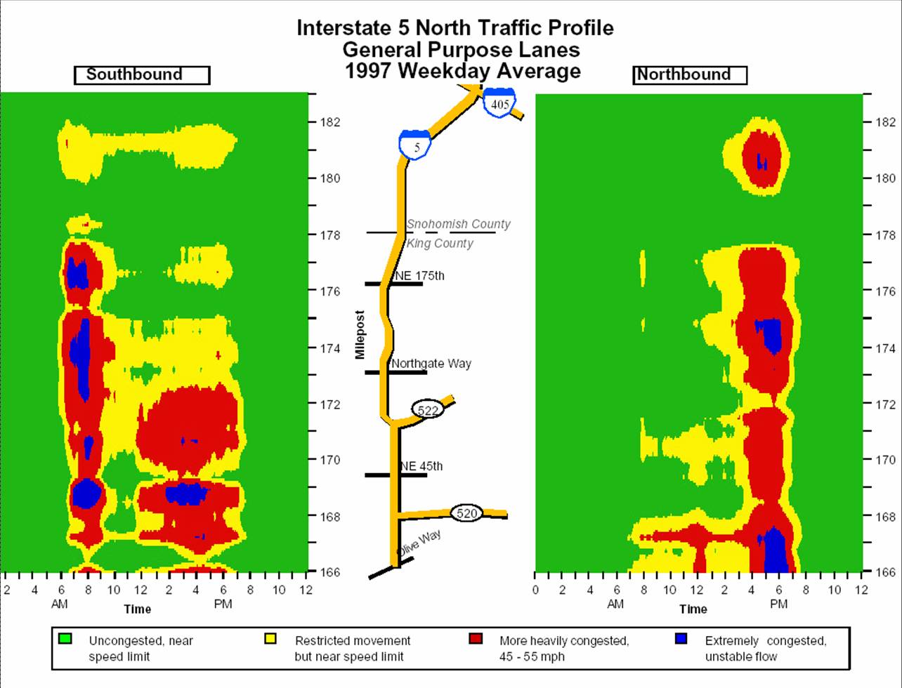
Figure 60 . Illustration. Washington State DOT traffic profile graph.(20)
Comparative summary tables are necessary to filter the information from the model run reports to the essential information necessary for making a decision. Table 17 shows a sample table used by Minnesota DOT (Mn/DOT) when comparing the results for existing (2005) conditions and two alternatives each for opening year (2015) and future year (2025).
Table 17 . Sample MOE summary table.
Analysis Segment |
Design Year |
|||||||
|---|---|---|---|---|---|---|---|---|
2005 |
2015 (Alt. A) |
2015 (Alt. B) |
2025 |
|||||
Speed1 |
Density2 |
Speed1 |
Density2 |
Speed1 |
Density2 |
Speed1 |
Density2 |
|
I-94 Merge to High Ridge Exit |
64 (64) |
11 (6) |
32 (64) |
34 (9) |
64 (64) |
15 (9) |
64 (64) |
16 (11) |
High Ridge Exit to High Ridge Entrance |
64 (64) |
10 (4) |
7 (64) |
111 (6) |
63 (64) |
14 (6) |
63 (64) |
13 (7) |
High Ridge Entrance to I-94 Diverge |
58 (63) |
12 (4) |
8 (62) |
108 (7) |
61 (64) |
15 (6) |
61 (63) |
17 (7) |
Notes: 1. Speed is expressed as mi/h.
2. Density is expressed as veh/lane/mi.
Table values are listed as XX (YY), where XX represents the a.m. peak average and YY represents the p.m. peak average.
Shaded cells represent where the average speed drops below 30 mi/h for any peak period for that alternative.
Figure 61 shows a sample graphic used by Mn/DOT for comparing the results for existing (2005) conditions, opening year (2015), and a future year (2025).
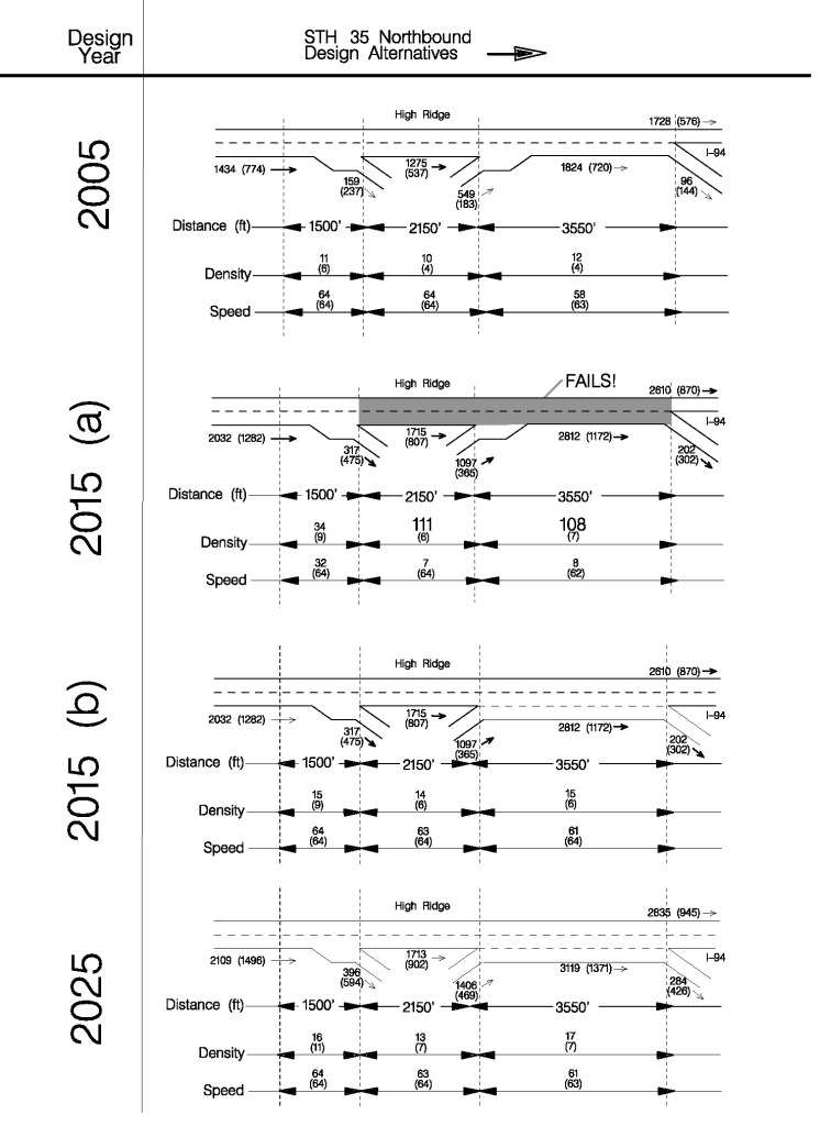
Figure 61 . Illustration. Sample comparison of project alternatives using schematic drawing.
6.7 Example Problem: Alternatives Analysis
The purpose of the alternatives analysis for this example problem (as continued from previous chapters) is to test various promising design scenarios and compare them to the no-build or base alternatives. As discussed in previous chapters, a CORSIM model was developed and calibrated to test the concept of widening HWY 100 and reconstructing the TH 7 and Minnetonka Boulevard interchanges. The complexity of the project resulted in the testing of numerous iterations of project alternatives. The alternative analysis process for the HWY 100 study included comparing the existing cloverleaf interchange to a diamond interchange at the HWY 100/TH 7 interchange, and analyzing numerous variations of a diamond interchange with frontage roads at the HWY 100/Minnetonka Boulevard interchange.
Prior to the modeling of alternatives, a number of design concepts were developed and screened down to a few viable alternatives. An alternative was deemed unviable if the basic geometric layout resulted in prohibitive right-of-way and/or environmental impacts.
Step 1: Baseline Demand Forecast
Traffic forecasts were prepared for the study area using the Regional Travel Demand model and manual post-processing techniques. The design year being considered for this project was 2031. Figure 62 shows an illustration of the resulting peak hour and daily baseline future demand forecasts for the HWY 100/TH 7 interchange area in 2031.
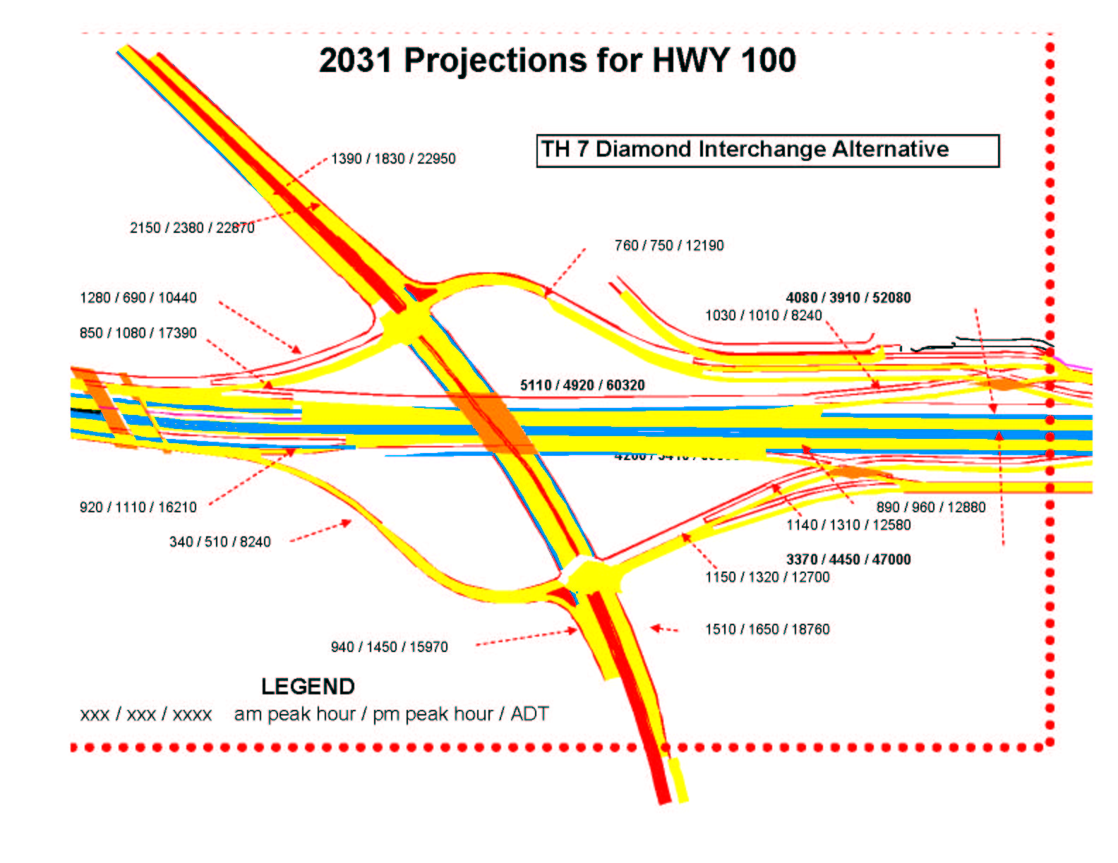
Figure 62 . Illustration. Example problem: traffic demand forecast at HWY 100/TH 7 interchange.
Step 2: Generation of Project Alternatives
The general process followed for generating and analyzing alternatives is shown in Figure 63. As shown in the figure, a large number of alternatives were considered initially and, for this project, they were analyzed at a high-level using sketch planning techniques. Various geometric layouts and concepts were developed and reviewed by all stakeholders in this stage. Due to right-of-way impacts, the desire to maintain access, and high construction costs, the alternative development and review process was extensive and took multiple years.
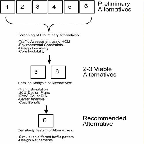
Figure 63 . Illustration. Example problem: alternatives generation and analysis process.
A small number of viable alternatives were then modeled and evaluated using CORSIM. The viable alternatives were then further screened down to a recommended alternative, which included adding mainline lanes on HWY 100, a cloverleaf interchange at TH 7, and diamond interchange at Minnetonka Boulevard. The CORSIM analysis was used to fine-tune these recommended alternatives and compare them to no-build or baseline conditions. Fine-tuning included modifying storage lengths, changing lane configurations, and adding auxiliary lanes.
Step 3: Selection of MOEs
The MOEs were discussed and agreed upon by all stakeholders involved in the process. The primary MOEs used for evaluating the freeway operations were:
- Mainline average density - expressed in vehicles per mile per lane. As density increases, freeway operations deteriorate, freedom to maneuver is more restricted, and operations become volatile and sensitive to any disruption, such as a lane change or entering ramp traffic.
- Mainline average speed – expressed miles per hour. The average vehicle speed was tabulated for each freeway segment over the analysis period, which serves as an indicator of the amount of congestion the mainline.
- Vehicles served – expressed as the number of vehicles that are actually able to pass through a given location in the network. Also referred to as throughput, this MOE serves as a comparison to the traffic volume demand at a location in the network. This MOE was tabulated for both the peak hour and entire analysis period, and it is related to density in that throughput decreases as density increases.
The primary MOEs used for evaluating the arterial operations were:
- Average control delay – expressed as seconds per vehicle. This MOE was tabulated for both individual approaches to a signalized intersection and for the intersection as a whole. As control delay increases, arterial operations deteriorate.
- Vehicles served – the same MOE as above for freeway operations, but on arterials it was tabulated for links at the approach to signalized intersections.
Step 4: Model Application
Before running CORSIM, the signal timing settings on the arterials were optimized using a commercial signal optimization software package. This step expedited the evaluation of arterial operations by developing optimized signal timings which were then used as input to the CORSIM model. Then, each CORSIM model alternative was run ten times with different random number seeds, and the MOEs from the five runs were averaged.
The traffic demand entering the re-construction area of HWY 100 at TH 7 and Minnetonka Boulevard exceeds the current capacity of the facilities surrounding the reconstruction area. The initial model runs of the proposed improvements indicated significant shortfalls in traffic at TH 7 and Minnetonka Boulevard. The proposed design capacity enhancements were made in the CORSIM model at the HWY 100/TH 62 and HWY 100/I-394 interchanges so traffic could both enter and exit the re-construction area. The improvements and capacity constraints outside of the reconstruction area could then be conveyed to the appropriate planning and programming officials for future considerations.
Step 5: Tabulation of Results
The model results for ten runs of each alternative were output into a spreadsheet and averaged for each alternative. With the capacity improvements modeled at the HWY 100/TH 62 and HWY 100/I-394 interchanges, there were no problems with queues extending beyond the study area or past the simulation analysis period. Overall, no post-model adjustments of untallied congestion were necessary.
The HWY 100/Minnetonka Boulevard interchange was considered for a new diamond interchange configuration and a new frontage road system. A total of six different alternatives were evaluated for this interchange. Table 18 shows the results of Alternative 1 (no-build) and Alternative 6 (one-way frontage road and ramp option).
Table 18 . Example problem: HWY 100/Minnetonka Blvd. interchange operations in 2031 .
Intersection |
App-roach |
Alternative 1 (No Build) |
Alternative 6 (Preferred) |
||||
|---|---|---|---|---|---|---|---|
Control delay: approach |
Control delay: inter-section |
Vehicles served: approach |
Control delay: approach |
Control delay: inter-section |
Vehicles served: approach |
||
Minnetonka Blvd/NB Ramp |
EB |
25 (23) |
87 (49) |
1178 (1393) |
15 (8) |
22 (17) |
1497 (1439) |
WB |
87 (47) |
1167 (1286) |
28 (19) |
1729 (1834) |
|||
SB |
81 (25) |
628 (1057) |
N/A |
N/A |
|||
NB |
187 (121) |
766 (912) |
22 (28) |
882 (994) |
|||
Minnetonka Blvd/SB Ramp |
WB |
22 (14) |
41 (30) |
801 (1453) |
9 (7) |
14 (12) |
962 (1466) |
EB |
41 (46) |
1400 (1520) |
17 (13) |
1736 (1578) |
|||
SB |
74 (29) |
462 (795) |
16 (17) |
586 (801) |
|||
Minnetonka Blvd/Lake St |
SB |
70 (23) |
77 (32) |
356 (373) |
19 (17) |
23 (16) |
400 (381) |
WB |
21 (16) |
703 (1388) |
21 (16) |
801 (1442) |
|||
NB |
85 (17) |
332 (418) |
14 (12) |
384 (421) |
|||
EB |
121 (67) |
878 (908) |
30 (19) |
1117 (956) |
|||
Vernon St/HWY 100 Off-Ramp |
NB |
2 (2) |
40 (1) |
78 (189) |
2 (2) |
1 (1) |
76 (194) |
SB |
57 (0) |
309 (373) |
0 (1) |
343 (376) |
|||
WB |
10 (4) |
80 (30) |
5 (5) |
80 (30) |
|||
Notes: EB = Eastbound, WB = Westbound, SB = Southbound, NB = Northbound.
N/A = Not applicable.
XX (YY) = AM peak hour (PM peak hour).
Control delay is expressed in seconds per vehicle.
Vehicles served is expressed in vehicles through the intersection approach in the peak hour.
Shaded cells represent where the control delay is greater than 55 seconds per vehicle for either peak hours.
The operations of the HWY 100 freeway were evaluated for the 2031 design year with a single lane added in each direction with and without various interchange improvement alternatives.
Table 19 shows the results for northbound HWY 100 without interchange improvements (baseline) and with the recommended interchange improvements for the HWY 100/TH 7 and HWY 100/Minnetonka Blvd interchanges. The MOE results in the table represent operations for the 2031 design year.
Table 19. Example problem: northbound HWY 100 freeway operations in 2031.
|
One Lane Added HWY 100, No Interchange Improvements |
One Lane Added HWY 100, All Recommended Interchange Improvements |
||||
|---|---|---|---|---|---|---|
Average Speed |
Average Density |
Vehicles Served |
Average Speed |
Average Density |
Vehicles Served |
|
1 |
62 (61) |
17 (23) |
11696 (15908) |
62 (58) |
14 (29) |
9736 (18437) |
2 |
62 (62) |
16 (22) |
10916 (15123) |
62 (59) |
13 (27) |
8631 (17219) |
3 |
48 (48) |
20 (25) |
12784 (16678) |
39 (38) |
21 (37) |
11316 (19538) |
4 |
61 (61) |
18 (21) |
11497 (14491) |
60 (59) |
15 (25) |
9435 (16263) |
5 |
60 (60) |
20 (23) |
13846 (17032) |
58 (56) |
20 (30) |
12795 (19878) |
6 |
61 (55) |
21 (26) |
14418 (17499) |
59 (58) |
20 (30) |
13617 (20560) |
7 |
62 (59) |
19 (22) |
12944 (15301) |
62 (61) |
17 (26) |
11505 (17512) |
8 |
60 (60) |
19 (20) |
13828 (16061) |
60 (59) |
18 (26) |
12770 (18673) |
9 |
58 (58) |
23 (24) |
14687 (16826) |
57 (46) |
22 (38) |
13968 (19721) |
10 |
61 (61) |
18 (18) |
11981 (14200) |
60 (56) |
18 (26) |
11101 (16667) |
11 |
44 (60) |
39 (19) |
10517 (11989) |
61 (60) |
18 (24) |
8637 (12766) |
12 |
18 (41) |
75 (30) |
12474 (14764) |
37 (48) |
35 (28) |
10580 (15513) |
13 |
18 (36) |
89 (42) |
11960 (13914) |
60 (60) |
18 (24) |
8412 (12549) |
14 |
21 (30) |
65 (48) |
13785 (16669) |
57 (53) |
23 (32) |
11188 (16192) |
15 |
27 (53) |
71 (33) |
13147 (15599) |
58 (59) |
22 (27) |
13571 (18375) |
16 |
26 (53) |
60 (28) |
13875 (16669) |
61 (61) |
19 (29) |
8938 (14867) |
17 |
23 (55) |
75 (32) |
13594 (15418) |
60 (60) |
16 (25) |
10099 (16564) |
18 |
33 (44) |
48 (38) |
15867 (17555) |
41 (37) |
21 (40) |
11873 (20711) |
19 |
51 (58) |
31 (29) |
13766 (15732) |
61 (58) |
14 (28) |
8629 (18188) |
20 |
62 (58) |
14 (19) |
9365 (12239) |
60 (46) |
13 (35) |
10440 (22242) |
21 |
60 (56) |
15 (20) |
10147 (13393) |
63 (57) |
14 (33) |
9218 (20900) |
22 |
49 (45) |
17 (25) |
11339 (16298) |
62 (57) |
14 (34) |
9807 (22521) |
Notes: Segments are numbered from the southern end of the HWY 100 study area to the northern end, with each segment representing a continuous section of northbound HWY 100 between ramps.
XX (YY) = AM peak hour (PM peak hour).
Average density is expressed in vehicles per mile per lane.
Vehicles served is expressed in vehicles through the segment in the peak period.
Shaded cells represent where the average density is greater than 38 veh/mi/lane for either of the peak hours.
Step 6: Evaluation of Alternatives
The evaluation of alternatives was prioritized to ensure that the freeway would operate sufficiently and the proposed interchange modifications would not negatively impact the freeway. A secondary goal was to ensure that the local streets operated acceptably. In order to prove the benefits of the reconstruction, the no-build scenario was evaluated for the 2031 design year and then compared to the various build alternatives. It was clear that under the no-build scenario, both the freeway and interchanges experienced significant delays and congestion (as highlighted in step 5 above).
A number of visual graphics were prepared to present the simulation results in a clear and concise manner. The graphics relayed the location and severity of “hot spot” locations to non-technical decision-makers. Figure 64 presents an example of these visual graphics, which consists of a comparison of the HWY 100/TH 7 interchange operations in 2031. The figure shows a schematic drawing of the no-build (existing cloverleaf interchange) and preferred (diamond interchange) alternatives, and specific segments were shaded where the operations will be unacceptable (decided to be when control delay exceeded 55 seconds per vehicle or average density exceeded 38 vehicles per mile per lane).
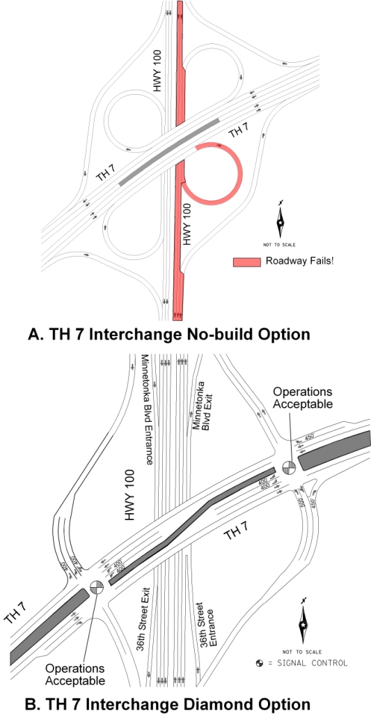
Figure 64 . Illustration. Example problem: visual comparison of HWY 100/TH 7 interchange alternatives.
Overall, the CORSIM analysis allowed for the testing of many alternatives, which helped decision-makers make a sound transportation investment decision in the end. The analysis that the recommended build scenario for HWY 100 achieved the goals of ensuring that the freeway functioned acceptably, with the proposed interchange configurations at the HWY 100/TH 7 and HWY 100/Minnetonka Boulevard interchanges having minimal impact to the freeway. The analysis also showed that the HWY 100/TH 7 interchange would function well from the local street perspective, but the HWY 100/Minnetonka Boulevard interchange required additional work to operate acceptably on the local streets.
The analysis also allowed a system-wide perspective to be taken on the HWY 100 corridor, which was useful because, through the CORSIM analysis, it was discovered that capacity expansions are needed just outside the re-construction area at the HWY 100/TH 62 and HWY 100/I-394 interchanges to adequately meet the 2031 demand forecasts.