| |
This section provides an overview of the technical aspects of microsimulation. It identifies and defines the terminology typically used, and what model types and procedures are generally employed in microsimulation. This section also provides a general introduction to traffic simulation models. Readers interested in additional details on the technical aspects of microsimulation may consult the Revised Monograph on Traffic Flow Theory (Chapter 10: Traffic Simulation) or other documents.
Simulation models are designed to emulate the behavior of traffic in a transportation network over time and space to predict system performance. Simulation models include the mathematical and logical abstractions of real-world systems implemented in computer software. Simulation model runs can be viewed as experiments performed in the laboratory rather than in the field.
Traffic simulation models describe the changes in the system state through discrete intervals in time. There are generally two types of models, depending on whether the update time intervals are fixed or variable:
Discrete Time (Time-Scan) Models: The system is being updated at fixed-time intervals. For example, the model calculates the vehicle position, speed, and acceleration at 1-s intervals. The choice of the update time interval depends on how accurately the system needs to be simulated at the expense of computer-processing time. Most microsimulation models employ a 0.1-s resolution for updating the system. Traffic systems are typically modeled using time-scan models because they experience a continuous change in state.
Discrete Event (Event-Scan) Models: In these models, the time intervals vary in length and correspond to the intervals between events. For example, a pre-timed traffic signal indication (e.g., green) remains constant for 30 s until its state changes instantaneously to yellow. The operation of the signal is described by recording its changes in state when events occur, rather than monitoring the state of the signal each second. Event-scanning models typically achieve significant reductions in computer run time. However, they are suitable for simulating systems whose states change infrequently.
Simulation models are typically classified according to the level of detail at which they represent the traffic stream. These include:
Microscopic Models: These models simulate the characteristics and interactions of individual vehicles. They essentially produce trajectories of vehicles as they move through the network. The processing logic includes algorithms and rules describing how vehicles move and interact, including acceleration, deceleration, lane changing, and passing maneuvers.
Mesoscopic Models: These models simulate individual vehicles, but describe their activities and interactions based on aggregate (macroscopic) relationships. Typical applications of mesoscopic models are evaluations of traveler information systems. For example, they can simulate the routing of individual vehicles equipped with in-vehicle, real-time travel information systems. The travel times are determined from the simulated average speeds on the network links. The average speeds are, in turn, calculated from a speed-flow relationship.
Macroscopic Models: These models simulate traffic flow, taking into consideration aggregate traffic stream characteristics (speed, flow, and density) and their relationships. Typically, macroscopic models employ equations on the conservation of flow and on how traffic disturbances (shockwaves) propagate in the system. They can be used to predict the spatial and temporal extent of congestion caused by traffic demand or incidents in a network; however, they cannot model the interactions of vehicles on alternative design configurations.
Microscopic models are potentially more accurate than macroscopic simulation models. However, they employ many more parameters that require calibration. Also, the parameters of the macroscopic models (e.g., capacity) are observable in the field. Most of the parameters of the microscopic models cannot be observed directly in the field (e.g., minimum distances between vehicles in car-following situations).
Simulation models are also classified by how they represent the randomness in the traffic flow, including:
Deterministic Models: These models assume that there is no variability in the driver-vehicle characteristics. For example, it is assumed that all drivers have a critical gap of 5 s in which to merge into a traffic stream, or all passenger cars have a vehicle length of 4.9 m (16 ft).
Stochastic Models: These models assign driver-vehicle characteristics from statistical distributions using random numbers. For example, the desired speed of a vehicle is randomly generated from an assumed normal distribution of desired speeds, with a mean of 105 km/h (65 mi/h) and a standard deviation of 8 km/h (5 mi/h). Stochastic simulation models have routines that generate random numbers. The sequence of random numbers generated depends on the particular method and the initial value of the random number (random number seed). Changing the random number seed produces a different sequence of random numbers, which, in turn, produces different values of driver-vehicle characteristics.
Stochastic models require additional parameters to be specified (e.g., the form and parameters of the statistical distributions that represent the particular vehicle characteristic). More importantly, the analysis of the simulation output should consider that the results from each model run vary with the input random number seed for otherwise identical input data. Deterministic models, in contrast, will always produce the same results with identical input data.
Microsimulation models employ several submodels, analytical relationships, and logic to model traffic flow. Detailed descriptions of each submodel are beyond the scope of this section. Instead, this document focuses on some key aspects of the simulation process that will probably affect the choice of the particular tool to be used and the accuracy of the results.
Simulation models include algorithms and logic to:
At the beginning of the simulation run, the system is empty. Vehicles are generated at the entry nodes of the analytical network, based on the input volumes and an assumed headway distribution. Suppose that the specified volume is V = 600 veh/h for a 15-min analytical period and that the model uses a uniform distribution of vehicle headways. Then, a vehicle will be generated at time intervals:
H = mean headway = 3600/V = 3600/600 = 6 s (Equation 8)
If the model uses the shifted negative exponential distribution to simulate the arrival of vehicles at the network entry node instead of the uniform distribution, then vehicles will be generated as time intervals:
![]() (Equation 9)
(Equation 9)
where:
h = headway (in seconds) separating each generated vehicle
hmin = specified minimum headway (e.g., 1.0 s)
R = random number (0 to 1.0)
When a vehicle is generated at the entry of the network, the simulation model assigns driver-vehicle characteristics. The following characteristics or attributes are commonly generated for each driver-vehicle unit:
Vehicle: Type (car, bus, truck), length, width, maximum acceleration and deceleration, maximum speed, maximum turn radius, etc.
Driver: Driver aggressiveness, reaction time, desired speed, critical gaps (for lane changing, merging, crossing), destination (route), etc.
Note that the different models may employ additional attributes for each driver-vehicle unit to ensure that the model replicates real-world conditions. Each attribute may be represented in the model by constants (e.g., all passenger cars have a vehicle length of 4.9 m (16 ft)), functional relationships (e.g., maximum vehicle acceleration is a linear function of its current speed), or probability distributions (e.g., driver's desired speed is obtained from a normal distribution). Most microsimulation models employ statistical distributions to represent the driver-vehicle attributes. The statistical distributions employed to represent the variability of the driver-vehicle attributes and their parameters must be calibrated to reflect local conditions.
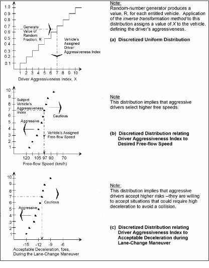
Figure 13 illustrates a generic process for generating driver-vehicle attributes for a stochastic microscopic simulation model. Drivers are randomly assigned an "aggressiveness index" ranging from 1 (very aggressive) to 10 (very cautious), drawn from a uniform distribution to represent the range of human behavior. Once the value of the aggressiveness has been assigned (X = 7 in this example), it is used to assign the value of the free-flow speed (97 km/h) and the acceptable deceleration (-3.4 m/s2 (-11 ft/s2)) from the corresponding distribution of speeds and accelerations.
Source: Traffic Flow Theory Monograph (Chapter 10: Simulation)
This section briefly describes the process for simulating vehicle movement and how it is impacted by the physical environment. The physical environment -- the transportation network under study -- is typically represented as a network of links and nodes. Links are one-way roadways with fixed design characteristics and nodes that represent intersections or locations where the design characteristics of the links change. Simulation models have different limits on the network size (maximum number of links and nodes).
Vehicles, in the absence of impedance from other vehicles, travel at their desired speed on the network links. However, their speed may be affected by the link-specified geometry (horizontal and vertical alignment), pavement conditions, and other factors. For example, the simulation model computes the actual vehicle speed as the minimum value from the desired speed and the speed computed for the specified vertical and horizontal alignment. However, not all microsimulation tools model the sensitivity of vehicle speeds to link design characteristics.
Vehicles proceed through the network until they exit the system at their destination. Typically, there are two types of simulation models: turning-fraction based or O-D based. In O-D-based models, the O-D matrix is input, and when a vehicle is generated at an origin, it is assigned its destination. The vehicle then exits the network at the specified destination. In turning-fraction-based models, the vehicle destination is randomly assigned at the entry of the link, based on specified turning volumes (or fractions) at the downstream end of the link. For example, for a vehicle entering a signalized intersection approach, the vehicle destination (going through or turning) is randomly determined based on the input turning-volume fractions for the particular link. This also implies that turning-fraction models are not well suited for tracing the performance of individual vehicles throughout the network and evaluating the effectiveness of certain ITS options (e.g., a fraction of vehicles being equipped with real-time information systems).
Simulation models employ a number of approaches to guide vehicles within the network. They typically employ warning signs to advise the simulated vehicle to change lanes because it needs to exit at the downstream off-ramp, its lane is ending, or there is a blockage downstream. The location of the warning signs may significantly affect the accuracy of the simulation. For example, vehicles traveling on the freeway at a speed of 97 km/h (60 mi/h) (27 m/s (88 ft/s)) may miss their exit without this advance warning if they are traveling in the median lane of a multilane freeway and are required to make multiple lane changes to exit at the downstream end of a short link.
Microscopic models simulate the interactions of individual vehicles as they travel in the analytical network using car-following, lane-changing, and queue discharge algorithms.
The interaction between a leader and follower pair of vehicles traveling in the same lane, is generally assumed to be a form of stimulus-response mechanism:
Response follower (t+T) = (sensitivity) • (stimulus) t (Equation 10)
where:
T = reaction time (time lag) for the response of the following vehicle
Car-following models for highway traffic were proposed since the inception of the traffic-flow theory in the early 1950s. Extensive experimentation and theoretical work were performed at the General Motors (GM) laboratories and elsewhere. Most of the existing simulation models employ fail-safe car-following algorithms. Such algorithms simulate car-following behavior by maintaining a minimum safe distance between vehicles subject to stochastically generated vehicle characteristics (e.g., maximum acceleration and deceleration rates). The fail-safe car-following algorithms currently implemented in most simulation models consist of the following components:
(Equation 11)
where:
af = acceleration of the following vehicle after a reaction time T
vl and vf = speeds of the leading and following vehicles, respectively
s = distance between vehicles
Xi = parameters specific to the particular car-following model
The modeling of lane changing is based on the gap-acceptance process. A vehicle may change lanes if the available gap in the target lane is greater than its critical gap. Typically, three types of lane changes are modeled:
These considerations are typically combined in a risk measure. More aggressive drivers would accept a higher risk value (i.e., shorter gaps and higher acceleration/deceleration rates) to change lanes. Moreover, the risk value may be further increased, depending on the type of lane change and the situation. For example, a merging vehicle reaching the end of the acceleration lane may accept much higher risk values (forced lane changes).
The model's lane-changing logic and parameters have important implications for traffic performance, especially for freeway merging and weaving areas. In addition, the time assumed for completion of the lane-change maneuver affects traffic performance because the vehicle occupies both lanes (original and target lanes) during this time interval. Furthermore, one lane change is allowed per simulation time interval.
Table of Contents | List of Tables | List of Figures | Top of Section | Previous Section | Next Section | HOME