| |
Project alternatives analysis is the sixth task in the microsimulation analysis process. It is the reason for developing and calibrating the microsimulation model. The lengthy model development process has been completed and now it is time to put the model to work.
The analysis of project alternatives involves the forecasting of the future demand for the base case and the testing of various project alternatives against this baseline future demand. The analyst must run the model several times, review the output, extract relevant statistics, correct for biases in the reported results, and perform various analyses of the results. These analyses may include hypothesis testing, computation of confidence intervals, and sensitivity analyses to further support the conclusions of the analysis.
The alternatives analysis task consists of several steps:
This step consists of establishing the future level of demand to be used as a basis for evaluating project alternatives.
Forecasts of future travel demand are best obtained from a travel demand model. These models require a great deal of effort and time to develop and calibrate. If one does not already exist, then the analyst may seek to develop demand forecasts based on historic growth rates. A trend-line forecast might be made, assuming that the recent percentage of growth in traffic will continue in the future. These trend-line forecasts are most reliable for relatively short periods of time (5 years or less). They do not take into account the potential of future capacity constraints to restrict the growth of future demand. Additional information and background regarding the development of traffic data for use in highway planning and design may be found in National Cooperative Highway Research Program (NCHRP) Report 255, Highway Traffic Data for Urbanized Area Project Planning and Design.
Regardless of which method is used to estimate future demand (regional model or trend line), care must be taken to ensure that the forecasts are a reasonable estimate of the actual amount of traffic that can arrive within the analytical period at the study area. Regional model forecasts are usually not well constrained to system capacity and trend-line forecasts are totally unconstrained. Appendix F provides a method for constraining future demands to the physical ability of the transportation system to deliver the traffic to the microsimulation model study area.
All forecasts are subject to uncertainty. It is risky to design a road facility to a precise future condition given the uncertainties in the forecasts. There are uncertainties in both the probable growth in demand and the available capacity that might be present in the future. Slight changes in the timing or design of planned or proposed capacity improvements outside of the study area can significantly change the amount of traffic delivered to the study area during the analytical period. Changes in future vehicle mix and peaking can easily affect capacity by 10 percent. Similarly, changes in economic development and public agency approvals of new development can significantly change the amount of future demand. Thus, it is good practice to explicitly plan for a certain amount of uncertainty in the analysis. This level of uncertainty is the purpose of sensitivity testing (explained in a separate section below).
In this step, the analyst generates improvement alternatives based on direction from the decision-makers and through project meetings. They will probably reflect operational strategies and/or geometric improvements to address the problems identified based on the baseline demand forecasts. The specifics of alternatives generation are beyond the scope of this report. Briefly, they consist of:
MOEs are the system performance statistics that best characterize the degree to which a particular alternative meets the project objectives (which were determined in the Project Scope task). Thus, the appropriate MOEs are determined by the project objectives and agency performance standards rather than what is produced by the model. This section, however, discusses what output is typically produced by microsimulation software so that the analyst can appreciate what output might be available for constructing the desired MOEs.
Microsimulation, by its very nature, can bury the analyst in detailed microscopic output. The key is to focus on a few key indicators of system performance and localized breakdowns in the system (locations where queues are interfering with systems operation).
As explained above, the selection of MOEs should be driven by the project objectives and the agency performance standards; however, many MOEs of overall system performance can be computed directly or indirectly from the following three basic system performance measures:
These three basic performance measures can also be supplemented with other model output, depending on the objectives of the analysis. For example, total system delay is a useful overall system performance measure for comparing the congestion-relieving effectiveness of various alternatives. The number of stops is a useful indicator for signal coordination studies.
In addition to evaluating overall system performance, the analyst should also be evaluating if and where there are localized system breakdowns ("hot spots"). A hot spot may be indicated by a persistent short queue that lasts too long, a signal phase failure (green time that fails to clear all waiting vehicles), or a blocked link (queue that backs up onto an upstream intersection).
A blocked link is the most significant indicator of localized breakdowns. A queue of vehicles that fills a link and blocks an upstream intersection can have a significant impact on system performance. A link queue overflow report can be developed to identify the links and times during the simulation period when the computed queue of vehicles equaled (and, therefore, probably actually exceeded) the storage capacity of the link.51
Signal phase failures, where the provided green time is insufficient to clear the queue, indicate potential operational problems if the queues continue to build over several cycles. The analyst should develop a signal phase failure report to indicate when and where signal green times are not sufficient to clear out all of the waiting queues of vehicles during each cycle.
At the finest level of detail, the analyst may wish to develop a report of the presence of persistent queues of a minimum length. This "hot spot" report would identify persistent queues on a lane-by-lane basis of a minimum number of vehicles that persist for a minimum amount of time. This report points the analyst to locations of persistent long queues (even those that do not overflow beyond the end of a link) during the simulation period.
Microsimulation models employ random numbers to represent the uncertainty in driver behavior in any given population of drivers. They will produce slightly different results each time they are run, with a different random number seed giving a different mix of driver behaviors. The analyst needs to determine if the alternatives should be evaluated based on their average predicted performance or their worst case predicted performance.
The average or mean performance is easy to compute and interpret statistically. The analyst runs the model several times for a given alternative, using different random number seeds each time. The results of each run are summed and averaged. The standard deviation of the results can be computed and used to determine the confidence interval for the results.
The worst case result for each alternative is slightly more difficult to compute. It might be tempting to select the worst case result from the simulation model runs; however, the difficulty is that the analyst has no assurance that if the model were to be run a few more times, the model might not get an even worse result. Thus, the analyst never knows if he or she has truly obtained the worst case result.
The solution is to compute the 95th percentile probable worst outcome based on the mean outcome and an assumed normal distribution for the results.52, 53 The equation below can be used to make this estimate:
![]() (Equation 5)
(Equation 5)
where:
m = mean observed result in the model runs
s = standard deviation of the result in the model runs
The calibrated microsimulation model is applied in this step to compute the MOEs for each alternative. Although model operation is adequately described in the software user's guide, there are a few key considerations to be taken into account when using a microsimulation model for the analysis of alternatives.
Microsimulation models rely on random numbers to generate vehicles, select their destination and route, and determine their behavior as they move through the network. No single simulation run can be expected to reflect any specific field condition. The results from individual runs can vary by 25 percent and higher standard deviations may be expected for facilities operating at or near capacity.54 It is necessary to run the model several times with different random number seeds55 to get the necessary output to determine mean, minimum, and maximum values. The analyst must then post-process the runs to obtain the necessary output statistics (see Appendix B for guidance on the computation of confidence intervals and the determination of the minimum number of repetitions of model runs).
The initialization (warmup) period before the system reaches equilibrium for the simulation period should be excluded from the tabulated statistics (see Appendix C for guidance on identifying the initialization period).
The simulation geographic and temporal limits should be sufficient to include all congestion related to the base case and all of the alternatives. Otherwise, the model will not measure all of the congestion associated with an alternative, thus causing the analyst to underreport the benefits of an alternative. See the subsection below on the methods for correcting congestion bias in the results.
The analyst should consider the potential impact of alternative improvements on the base case forecast demand. This should take into consideration the effects of a geometric alternative, an operational strategy, and combinations of both. The analyst should then make a reasonable effort to incorporate any significant demand effects within the microsimulation analysis.56
Most simulation models do not currently optimize signal timing or ramp meter controls. Thus, if the analyst is testing various demand patterns or alternatives that significantly change the traffic flows on specific signalized streets or metered ramps, he or she may need to include a signal and meter control optimization substep within the analysis of each alternative. This optimization might be performed offline using a macroscopic signal timing or ramp metering optimization model. Or, the analyst may run the simulation model multiple times with different signal settings and manually seek the signal setting that gives the best performance.
Microsimulation models typically produce two types of output: (1) animation displays and (2) numerical output in text files.57 The animation display shows the movement of individual vehicles through the network over the simulation period. Text files report accumulated statistics on the performance of the network. It is crucial that the analyst reviews both numerical and animation output (not just one or the other) to gain a complete picture of the results.58 This information can then be formatted for inclusion in the final report.
Animation output is powerful in that it enables the analyst to quickly see and qualitatively assess the overall performance of the alternative. However, the assessment can only be qualitative. In addition, reviewing animation results can be time-consuming and tedious for numerous model repetitions, large networks, and long simulation periods. The analyst should select one or more model run repetitions for review and then focus his or her attention on the key aspects of each animation result.
The analyst has to decide whether he or she will review the typical case output, or the worst case output, or both. The typical case might give an indication of the average conditions for the simulation period. The worst case is useful for determining if the transportation system will experience a failure and for viewing the consequences of that failure.
The next question that the analyst must decide is how to identify which model repetition represents typical conditions and which repetition reflects worst case conditions. The total VHT may be a useful indicator of typical and worst case conditions. The analyst might also select other measures, such as the number of occurrences of blocked links (links with queue overflows) or delay.
If VHT is selected as the measure and the analyst wishes to review the typical case, then he or she would pick the model run repetition that had the total VHT that came closest to falling within the median of the repetitions (50 percent of the repetitions had a VHT less than that, and 50 percent has more VHT). If the analyst wished to review the worst case, then he or she would select the repetition that had the highest VHT.
The pitfall of using a global summary statistic (such as VHT) to select a model run repetition for review is that overall average system conditions does not mean that each link and intersection in the system is experiencing average conditions. The median VHT repetition may actually have the worst performance for a specific link. If the analyst is focused on a specific link or intersection, then he or she should select some statistic related to vehicle performance on that specific link or intersection for selecting the model run repetition for review.
The key event to look for in reviewing animation is the formation of persistent queues. Cyclical queues at signals that clear each cycle are not usually as critical unless they block some other traffic movement. The analyst should not confuse the secondary impact of queues (one queue blocking upstream movement and creating a secondary queue) with the root cause of the queuing problem. Eliminating the cause of the first or primary queue may eliminate all secondary queuing. Thus, the analyst should focus on the few minutes just prior to formation of a persistent queue to identify the causes of the queuing.
Microsimulation software reports the numerical results of the model run in text output files called "reports." Unless the analyst is reviewing actual vehicle trajectory output, the output reports are almost always a summary of the vehicle activity simulated by the model. The results may be summarized over time and/or space. It is critical that the analyst understands how the software has accumulated and summarized the results to avoid pitfalls in interpreting the numerical output.
Microsimulation software may report instantaneous rates (such as speed) observed at specific instances of time, or may accumulate the data over a longer time interval and either report the sum, the maximum, or the average. Depending on the software program, vehicle activity that occurs between time steps (such as passing over a detector) may not be tallied, accumulated, or reported.
Microsimulation software may report the results for specific points on a link in the network or aggregated for the entire link. The point-specific output is similar to what would be reported by detectors in the field. Link-specific values of road performance are accumulated over the length of the link and, therefore, will vary from the point data.
The key to correctly interpreting the numerical output of a microsimulation model is to understand how the data were accumulated by the model and summarized in the report. The report headings may give the analyst a clue as to the method of accumulation used; however, these short headings cannot usually be relied on. The method of data accumulation and averaging can be determined through a detailed review of the model documentation of the reports that it produces, and, if the documentation is lacking, by querying the software developers themselves.
An initial healthy skepticism is valuable when reviewing reports until the analyst has more experience with the software. It helps to cross-check output to ensure that the analyst understands how the data is accumulated and reported by the software.
To make a reliable comparison of the alternatives, it is important that vehicle congestion for each alternative be accurately tabulated by the model. This means that congestion (vehicle queues) should not extend physically or temporally beyond the geographic or temporal boundaries of the simulation model. Congestion that overflows the time or geographic limits of the model will not normally be reported by the model, which can bias the comparison of alternatives.
The tabulated results should also exclude the initial and unrealistic initialization period when vehicles are first loaded on the network.
Ideally, the simulation results for each alternative would have the following characteristics:
It may not always be feasible to achieve all three of these conditions, so it may be necessary to adjust for congestion that is missing from the model tabulations of the results.
If simulation alternatives are severely congested, then the simulation may be unable to load vehicles onto the network. Some may be blocked from entering the network on the periphery. Some may be blocked from being generated on internal links. These blocked vehicles will not typically be included in the travel time (VHT) or delay statistics for the model run.59 The best solution is to extend the network back to include the maximum back of the queue. If this is not feasible, then the analyst should correct the reported VHT to account for the unreported delay for the blocked vehicles.
Microsimulation software will usually tally the excess queue that backs up outside the network as "blocked" vehicles (vehicles unable to enter the network) for each time step. The analyst totals the number of software-reported blocked vehicles for each time step of the simulation and multiplies this figure by the length of each time step (in hours) to obtain the vehicle-hours of delay. The delay resulting from blocked vehicles is added to the model-reported VHT for each model run.
Vehicles queues that are present at the end of the simulation period may affect the accumulation of total delay and distort the comparison of alternatives (cyclical queues at signals can be neglected). The "build" project alternative may not look significantly better than the "no-build" option if the simulation period is not long enough to capture all of the benefits. The best solution is to extend the simulation period until all of the congestion that built up over the simulation period is served. If this is not feasible, the analyst can make a rough estimate of the uncaptured residual delay by computing how many vehicle-hours it would take to clear the queue using the equation given below:
![]() (Equation 6)
(Equation 6)
where:
VHT(Q) = extra VHT of delay attributable to a queue present at the end of the simulation period
Q = number of vehicles remaining in the queue at the end of the simulation period
C = discharge capacity of the bottleneck in veh/h
The equation computes the area of the triangle created by the queue and the discharge capacity after the end of the simulation period (see Figure 11):
Note that this is not a complete estimate of the residual delay since it ignores the interaction of vehicles left over from the simulation period that interfere with traffic arriving during later time periods.
This step involves the evaluation of alternatives using the microsimulation model results. First, the interpretation of system performance results is discussed. Then, various analyses are discussed for assessing the robustness of the results. The ranking of alternatives and cost-effectiveness analyses are well documented in other reports and are not discussed here.
This subsection explains how to interpret the differences between alternatives for the three basic system performance measures (VMT, VHT, and system speed).
VMT provides an indication of total travel demand (in terms of both the number of trips and the length of the trips) for the system.60 Increases in VMT generally indicate increased demand (car, bus, and truck). VMT is computed as the product of the number of vehicles traversing a link and the length of the link, summed over all links. Since VMT is computed as a combination of the number of vehicles on the system and their length of travel, it can be influenced both by changes in the number of vehicles and changes in the trip lengths during the simulation period. The following can cause changes in VMT between one alternative and the next:
VHT provides an estimate of the amount of time expended traveling on the system.61 Decreases in VHT generally indicate improved system performance and reduced traveling costs for the public. VHT is computed as the product of the link volume and the link travel time, summed over all links. Since VHT is computed as a combination of the number of vehicles and the time spent traveling, it can be influenced both by changes in demand (the number of vehicles) and changes in congestion (travel time). Changes in VHT between one alternative and the next can be caused by the following:
Mean system speed is an indicator of overall system performance. Higher speeds generally indicate reduced travel costs for the public. The mean system speed is computed from the VMT and VHT as follows:
Mean System Speed = VMT/VHT (Equation 7)
Changes in the mean system speed between one alternative and the next can be caused by the following:
Total system delay, if available, is useful because it reports the portion of total travel time that is most irritating to the traveling public. However, defining "total system delay" can be difficult. It depends on what the analyst or the software developer considers to be ideal (no delay) travel time. Some sources consider delay to include only the delay caused by increases in demand above some base uncongested (free-flow) condition. Others add in the base delay occurring at traffic control devices, even at low-flow conditions. Some include acceleration and deceleration delay. Others include only stopped delay. The analyst should consult the software documentation to ensure the appropriate use and interpretation of this measurement of system performance.
When the microsimulation model is run several times for each alternative, the analyst may find that the variance in the results for each alternative is close to the difference in the mean results for each alternative. How is the analyst to determine if the alternatives are significantly different? To what degree of confidence can the analyst claim that the observed differences in the simulation results are caused by the differences in the alternatives and not just the result of using different random number seeds? This is the purpose of statistical hypothesis testing. Hypothesis testing determines if the analyst has performed an adequate number of repetitions for each alternative to truly tell the alternatives apart at the analyst's desired level of confidence. Hypothesis testing is discussed in more detail in Appendix E.
Confidence intervals are a means of recognizing the inherent variation in microsimulation model results and conveying them to the decision-maker in a manner that clearly indicates the reliability of the results. For example, a confidence interval would state that the mean delay for alternative x lies between 35.6 s and 43.2 s, with a 95-percent level of confidence. If the 95-percent confidence interval for alternative y overlaps that of x, the decision-maker would consider the results to be less favorable for either alternative. They could be identical. Computation of the confidence interval is explained in Appendix B.
A sensitivity analysis is a targeted assessment of the reliability of the microsimulation results, given the uncertainty in the input or assumptions. The analyst identifies certain input or assumptions about which there is some uncertainty and varies them to see what their impact might be on the microsimulation results.
Additional model runs are made with changes in demand levels and key parameters to determine the robustness of the conclusions from the alternatives analysis. The analyst may vary the following:
A sensitivity analysis of different demand levels is particularly valuable when evaluating future conditions. Demand forecasts are generally less precise than the ability of the microsimulation model to predict their impact on traffic operations. A 10-percent change in demand can cause a facility to go from 95 percent of capacity to 105 percent of capacity, with a concomitant massive change in the predicted delay and queuing for the facility. The analyst should estimate the confidence interval for the demand forecasts and test the microsimulation at the high end of the confidence interval to determine if the alternative still operates satisfactorily at the potentially higher demand levels.
The analyst should plan for some selected percentage above and below the forecasted demand to allow for these uncertainties in future conditions. The analyst might consider at least a 10-percent margin of safety for the future demand forecasts. A larger range might be considered if the analyst has evidence to support the likelihood of greater variances in the forecasts.
To protect against the possibility of both underestimates and overestimates in the forecasts, the analyst might perform two sensitivity tests -- one with 110 percent of the initial demand forecasts and the other with 90 percent of the initial demand forecasts -- for establishing a confidence interval for probable future conditions.62
Street improvements assumed to be in place outside the simulation study area can also have a major impact on the simulation results by changing the amount of traffic that can enter or exit the facilities in the study area. Sensitivity testing would change the assumed future level of demand entering the study area and the assumed capacity of facilities leaving the study area to determine the impact of changes in the assumed street improvements.
The analyst may also run sensitivity tests to determine the effects of various assumptions about the parameter values used in the simulation. If the vehicle mix was estimated, variations in the percentage of trucks might be tested. The analyst might also test the effects of different percentages of familiar drivers in the network.
It is often valuable when explaining microsimulation model results to the general public to report the results in terms of HCM levels of service. However, the analyst should be well aware of the differences between the HCM and the microsimulation analysis when making these comparisons.
Delay is used in the HCM to estimate the LOS for signalized and unsignalized intersections. There are distinctions in the ways microsimulation software and the HCM define delay and accumulate it for the purpose of assessing LOS.
The HCM bases its LOS grades for intersections on estimates of mean control delay for the highest consecutive 15-min period within the hour. If microsimulation output is to be used to estimate LOS, then the results for each run must be accumulated over a similar 15-consecutive-minute time period and averaged over several runs with different random number seeds to achieve a comparable result.
This still may not yield a fully comparable result, because all microsimulation models assign delay to the segment in which it occurs. For example, the delay associated with a single approach to a traffic signal may be parceled out over several upstream links if the queues extend beyond one link upstream from the intersection. Thus, when analysts seek to accumulate the delay at a signal, they should investigate whether the delay/queues extend beyond the single approach links to the signal.
Finally, the HCM does not use total delay to measure signal LOS. It uses "control delay." This is the component of total delay that results when a control signal causes a lane group to reduce speed or to stop. It is measured by comparison with the uncontrolled condition. The analyst needs to review the software documentation and seek additional documentation from the software vendor to understand how delay is computed by the software.
If microsimulation model reports of vehicle density are to be reported in terms of their LOS implications, it is important to first translate the densities reported by the software into the densities used by the HCM to report LOS for uninterrupted flow facilities.63
HCM 2000 defines freeway and highway LOS based on the average density of passenger car equivalent vehicles in a section of highway for the peak 15-min period within an hour. For ramp merge and diverge areas, only the density in the rightmost two lanes is considered for LOS. For all other situations, the density across all lanes is considered. Trucks and other heavy vehicles must be converted to passenger car equivalents using the values contained in the HCM according to vehicle type, facility type, section type, and grade.
HCM 2000 defines a queue as: "A line of vehicles, bicycles, or persons waiting to be served by the system in which the flow rate from the front of the queue determines the average speed within the queue. Slowly moving vehicles or people joining the rear of the queue are usually considered part of the queue." These definitions are not implementable within a microsimulation environment since "waiting to be served" and "slowly" are not easily defined. Consequently, alternative definitions based on maximum speed, acceleration, and proximity to other vehicles have been developed for use in microsimulation.
Note also that for most microsimulation programs, the number of queued vehicles counted as being in a particular turn-pocket lane or through lane cannot exceed the storage capacity of that lane. Any overflow is reported for the upstream lane and link where it occurs, not the downstream cause of the queue. Unlike macroscopic approaches that assign the entire queue to the bottleneck that causes it, microsimulation models can only observe the presence of a queue; they currently do not assign a cause to it. So, to obtain the 95-percent queue length, it may be necessary to temporarily increase the length of the storage area so that all queues are appropriately tallied in the printed output.
The same example problem from the previous chapters is continued here. The task now is to apply the calibrated model to the analysis of the ramp metering project and its alternatives.
A 5-year forecast was estimated using a straight-line growth approach assuming 2 percent growth per year uncompounded. The result was a forecasted 10-percent increase in traffic demand for the corridor. The forecasted growth for individual links and ramps varied from this average value.
Since the existing conditions were uncongested and the growth forecast is a modest 10 percent growth, the forecasted demand was not constrained because of anticipated capacity constraints on the entry links to the corridor.
Since a 5-year forecast is being performed, it was considered to be fairly reliable for such a short time period. No extra allowance was added to the forecasts or subtracted from them to account for uncertainty in the demand forecasts.
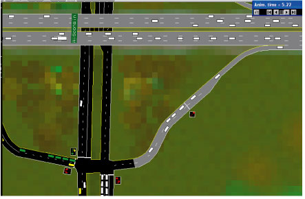
Two alternatives will be tested with the calibrated model -- no-build and build. The build alternative consists of ramp metering on the two eastbound freeway on-ramps. The no-build alternative has no ramp metering. Figure 12 illustrates the coding of one of the ramp meters.
The following system MOEs were selected for evaluation of the alternatives: VMT, VHT, and delay (vehicle-hours). The selected indicator of localized problems was a "blocked link," indicating that the queue filled up and overflowed the available storage in the link.
It was opted to report the mean results rather than the 95-percent worst case results.
The model was run 10 times for each alternative. The results were output into a spreadsheet and averaged for each alternative.
The impact of ramp meters on route choice was estimated outside of the model using a regional travel demand model to predict the amount of diversion. The regional model predicted that diversion was implemented in the simulation model by manually adjusting the turn percentages at the appropriate upstream intersections and ramp junctions.
The initialization period was automatically excluded from the tabulated results by the selected software program.
The results were reviewed to determine if building queues64 were extending beyond the physical boundaries of the model or the temporal boundaries of the analytical period. None was found, so it was not necessary to correct the model results for untabulated congestion.
Because of the modest differences in congestion between the alternatives, induced demand was not considered to be a significant factor in this analysis. No adjustments were made to the baseline demand forecasts.
Signal/meter control optimization was performed outside of the model using macroscopic signal optimization software and ramp meter optimization software. The recommended optimal settings were input into the simulation model. Separate optimizations were performed for the no-build and build alternatives.
The model results for 10 repetitions of each alternative were output into a spreadsheet and averaged for each alternative (see Table 7). A review of the animation output indicated that post-model corrections of untallied congestion were not necessary.65
Measure of Effectiveness |
Existing |
Future: No-Build |
Future: Build |
|---|---|---|---|
VMT: Freeway |
35,530 |
39,980 |
40,036 |
VMT: Arterial |
8,610 |
9,569 |
9,634 |
VMT: Total |
44,140 |
49,549 |
49,670 |
VHT: Freeway |
681.6 |
822.3 |
834.2 |
VHT: Arterial |
456.5 |
538.5 |
519.5 |
VHT: Total |
1138.1 |
1360.8 |
1353.7 |
Delay (VHT): Freeway |
33.1 |
90.4 |
101.0 |
Delay (VHT): Arterial |
214.3 |
269.7 |
248.9 |
Delay (VHT): Total |
247.4 |
360.1 |
349.9 |
Under the no-build scenario, the total delay on the corridor increased by 46 percent over existing conditions. The VMT increased by 12 percent and the total travel time increased by 20 percent. Most of the delay increases were on the freeway mainline links.
Under the improved scenario (ramp metering plus signal optimization), systemwide delay was reduced by about 3 percent (from the no-build scenario) with a slight increase in VMT.66 Freeway mainline traffic conditions improved at the expense of the on-ramp traffic.
The improvements are operationally acceptable (no spillbacks from the ramp meters to the arterial network).
Table of Contents | List of Tables | List of Figures | Top of Section | Previous Section | Next Section | HOME