Empirical Studies on Traffic Flow in Inclement Weather

5.0 Study Results

The research reported in this chapter quantifies the impact of inclement weather on traffic stream behavior by developing weather adjustment factors for key traffic stream parameters. These parameters include the free-flow speed, speed-at-capacity, capacity, and jam-density using data from three different cities in the U.S. The quality of these parameter estimates for a particular condition has a significant impact on the ability to discern changes in this parameter for different conditions. Furthermore, the automation of the parameter extraction process is critical in this situation because of the volume of data involved and the potential bias in manual fits. Consequently, an automated calibration procedure to estimate the key traffic stream parameters is utilized.

Initially, the traffic stream functional form and the calibration procedure are described briefly. Subsequently, the loop detector and weather data are described followed by the results and conclusions of the study.

5.1 Study Results

Having computed weather adjustment factors for three key traffic stream parameters (u_f, u_c, and q_c), a regression analysis was utilized to build a model that predicts the weather adjustment factor (WAF) for a given precipitation type (rain and snow), intensity level, and visibility level for each of the three key traffic stream parameters (u_f, u_c, and q_c), as illustrated in Figure 5.1.

Figure 5.1 Statistical Analysis Overview

[D]

The general model that was considered was of the form:

[6]

where F is the WAF, i is the precipitation intensity (cm/h), v is the visibility (km), (vi) is the interaction term between visibility and precipitation intensity, and c₁, c₂, c₃, c₄, c₅ and c₆ are calibrated model coefficients. In all models the interaction term was found to be insignificant and thus is not discussed further in the analysis.

The analysis was started by creating the correlation coefficient matrix. This first step along with ANOVA test was performed to assist in the selection of the variables to build the regression model.

A stepwise regression analysis was performed using the Minitab software (MINITAB). Stepwise regression removes and adds variables to the regression model for the purpose of identifying a useful subset of predictors. The coefficients and statistics for the best model for each dataset were generated by running the stepwise regression tool. Recognizing that automatic procedures cannot take into account the specific knowledge the analyst may have about the data, a validity check was made. This validity check ensured that the data did not produce unrealistic trends (e.g., the weather adjustment factors increased as the precipitation intensity increased). While such a model may be the best from a statistical standpoint, that may not be the case from a practical standpoint. In these rare cases, the model was constrained to ensure that it produced realistic trends.

The following step involved a check of both the model and variable significance. The model significance was checked through an Analysis of Variance (ANOVA) test. The null hypothesis (H₀) was that all model parameters were zero (i.e., c₂ =…= cn = 0), where n is the number of model parameters, while the alternative hypothesis (H₁) was that the model parameters were not zero c_j ¹0, for at least one j. Table 5.1 presents the results for the ANOVA test for the Twin Cities free-flow speed model (Rain).

Table 5.1 ANOVA Test Results for Free-Flow Speed (Rain – Twin Cities)

Source of Variation	DF	Sum of Square	Mean Square	F0	P-value
Regression	1	0.01128	0.01128	52.63	0.000
Error	43	0.00921	0.000214	[no value]	[no value]
Total	44	0.02049	[no value]	[no value]	[no value]

Since the P-value = 0.000<0.05, it was concluded that at least some of the model parameters (c₂,…,c_n) were not equal to zero. It should be noted here that the results of the stepwise regression, in terms of variables that should be included in the model, coincided with those of the previous step.

An imperative part of assessing the adequacy of a regression model is the significance of the individual regression coefficients. This test is important in determining the potential value of each of the independent variables. The null hypothesis that was tested was that the individual regression coefficients (c_j) were zero (H₀: c_j = 0 and H₁: c_j ≠ 0). A P-value greater than a (in this case 0.05) – presented within parenthesis under each coefficient in the table – meant that the null hypothesis could be accepted, implying that the independent variable x_j was insignificant and thus could be deleted from the model. The various models that were developed for the three parameters u_f, u_c, and q_c are summarized in Table 5.2, 5.3, and 5.5, respectively.

Table 5.2 Free-Flow Speed Regression Analysis Summary Results

Precip.	City	n	Coefficient Value (p-value) c1	Coefficient Value (p-value) c2	Coefficient Value (p-value) c3	Coefficient Value (p-value) c4	Coefficient Value (p-value) c5	Coefficient Value (p-value) c6	P-value	R2Adj	Normality Test: A2	Normality Test: P-value	Levene Variance Test
Rain	Baltimore	32	0.963 (0.00)	-0.333 (0.001)	[no value]	[no value]	[no value]	[no value]	0.001	0.304	0.485	0.211	0.684
Rain	Twin Cities	45	0.980 (0.000)	-0.0274 (0.000)	[no value]	[no value]	[no value]	[no value]	0.000	0.540	0.553	0.146	0.424
Rain	Seattle	43	0.973 (0.000)	-0.0650 (0.000)	0.0240 (0.004)	[no value]	0.0010 (0.044)	[no value]	0.000	0.607	0.336	0.493	0.067
Rain	Aggregate	111	0.981 (0.000)	-0.050 (0.000)	0.014 (0.011)	[no value]	[no value]	[no value]	0.000	0.734	0.646	0.089	0.168
Snow	Baltimore	8	0.955	[no value]	[no value]	[no value]	[no value]	[no value]	[no value]	[no value]	[no value]	[no value]	[no value]
Snow	Twin Cities	32	0.842 (0.000)	-0.31 (0.002)	[no value]	[no value]	0.0055 (0.000)	[no value]	0.000	0.866	0.456	0.251	0.704
Snow	Aggregate	40	0.838 (0.000)	-0.0908 (0.025)	[no value]	[no value]	0.00597 (0.000)	[no value]	0.000	0.824	0.340	0.482	0.624

Note: Minitab reports a P-value of less than 0.0005 as 0.000.

 

Table 5.3 Ratio of Speed-at-Capacity to Free-Flow Speed Analysis Summary Results

Precip.	City	n	Coefficient Value (p-value) c1	Coefficient Value (p-value) c2	Coefficient Value (p-value) c3	Coefficient Value (p-value) c4	Coefficient Value (p-value) c5	Coefficient Value (p-value) c6	P-value	R2Adj	Normality Test: A2	Normality Test: P-value	Levene Variance Test
Rain	Baltimore	35	0.936	[no value]	[no value]	[no value]	[no value]	[no value]	[no value]	[no value]	[no value]	[no value]	[no value]
Rain	Twin Cities	53	0.978	[no value]	[no value]	[no value]	[no value]	[no value]	[no value]	[no value]	[no value]	[no value]	[no value]
Rain	Seattle	50	0.940	[no value]	[no value]	[no value]	[no value]	[no value]	[no value]	[no value]	[no value]	[no value]	[no value]
Rain	Aggregate	138	[no value]	[no value]	[no value]	[no value]	[no value]	[no value]	[no value]	[no value]	[no value]	[no value]	[no value]
Snow	Baltimore	8	1.000	[no value]	[no value]	[no value]	[no value]	[no value]	[no value]	[no value]	[no value]	[no value]	[no value]
Snow	Twin Cities	41	1.000	[no value]	[no value]	[no value]	[no value]	[no value]	[no value]	[no value]	[no value]	[no value]	[no value]
Snow	Aggregate	[no value]	[no value]	[no value]	[no value]	[no value]	[no value]	[no value]	[no value]	[no value]	[no value]	[no value]	[no value]

Note: Minitab reports a P-value of less than 0.0005 as 0.000.

 

Table 5.4 Speed-at-Capacity Analysis Summary Results

Precip.	City	n	Coefficient Value (p-value) c1	Coefficient Value (p-value) c2	Coefficient Value (p-value) c3	Coefficient Value (p-value) c4	Coefficient Value (p-value) c5	Coefficient Value (p-value) c6	P-value	R2Adj	Normality Test: A2	Normality Test: P-value	Levene Variance Test
Rain	Baltimore	35	0.920 (0.00)	-0560 (0.003)	[no value]	[no value]	[no value]	[no value]	0.003	0.236	0.581	0.120	0.989
Rain	Twin Cities	53	0.928	[no value]	[no value]	[no value]	[no value]	[no value]	[no value]	[no value]	[no value]	[no value]	[no value]
Rain	Seattle	50	0.906	[no value]	[no value]	[no value]	[no value]	[no value]	[no value]	[no value]	[no value]	[no value]	[no value]
Rain	Aggregate	138	0.909	[no value]	[no value]	[no value]	[no value]	[no value]	[no value]	[no value]	[no value]	[no value]	[no value]
Snow	Baltimore	8	0.956	[no value]	[no value]	[no value]	[no value]	[no value]	[no value]	[no value]	[no value]	[no value]	[no value]
Snow	Twin Cities	41	0.852 (0.000)	[no value]	[no value]	0.0226 (0.000)	[no value]	[no value]	0.000	0.497	[no value]	0.828	0.864
Snow	Aggregate	47	0.816 (0.000)	[no value]	[no value]	0.0308 (0.000)	[no value]	[no value]	0.000	0.362	[no value]	[no value]	0.920

Note: Minitab reports a P-value of less than 0.0005 as 0.000.

 

Table 5.5 Capacity Analysis Summary Results

Precip.	City	n	Coefficient Value (p-value) c1	Coefficient Value (p-value) c2	Coefficient Value (p-value) c3	Coefficient Value (p-value) c4	Coefficient Value (p-value) c5	Coefficient Value (p-value) c6	P-value	R2Adj	Normality Test: A2	Normality Test: P-value	Levene Variance Test
Rain	Baltimore	35	0.892	[no value]	[no value]	[no value]	[no value]	[no value]	[no value]	[no value]	[no value]	[no value]	[no value]
Rain	Twin Cities	43	0.889	[no value]	[no value]	[no value]	[no value]	[no value]	[no value]	[no value]	[no value]	[no value]	[no value]
Rain	Seattle	49	0.896	[no value]	[no value]	[no value]	[no value]	[no value]	[no value]	[no value]	[no value]	[no value]	[no value]
Rain	Aggregate	137	0.892	[no value]	[no value]	[no value]	[no value]	[no value]	[no value]	[no value]	[no value]	[no value]	[no value]
Snow	Baltimore	6	0.877 (0.000)	[no value]	[no value]	[no value]	[no value]	[no value]	[no value]	[no value]	[no value]	[no value]	[no value]
Snow	Twin Cities	38	0.794 (0.000)	[no value]	[no value]	[no value]	0.00508 (0.000)	[no value]	0.000	0.480	0.318	0.524	0.859
Snow	Aggregate	45	0.792 (0.000)	[no value]	[no value]	[no value]	0.00480 (0.000)	[no value]	0.000	0.503	0.461	0.248	0.627

Note: Minitab reports a P-value of less than 0.0005 as 0.000.

Once the model and variable significance was established a screening of outlier data was applied. The screening approach involved removing data outside the 95 percent confidence limits using Minitab’s built-in data screening procedures. This data screening only involved the removal of a limited number of observations, which explains the slightly different number of data points for the same weather scenarios within Table 5.2, 5.3, and 5.5.

Regression analysis assumes that the residuals are normally and independently distributed with constant variance. Consequently, a normality and equal variance test was conducted on the residuals. The normality test hypothesized that the data were normally distributed (null hypothesis). A P-value that was less than the chosen a-value of 0.05 implied that the data might not be normally distributed. Figure 5.2 presents a normal probability plot for the residuals calculated for a sample model, the plot also shows the Anderson-Darling goodness-of-fit test results. The Anderson-Darling statistic is a measure of how far the data points fall from the fitted normal line. The statistic is a weighted squared distance from the plot points to the fitted line with larger weights in the tails of the distribution. A smaller Anderson-Darling statistic indicates that the distribution fits the data better. The Anderson-Darling test’s p-value (column before last) (0.553>>0.05) indicates that there was no evidence that the residuals were not normally distributed. As summarized in Table 5.2, 5.3, and 5.5 all data sets provided no evidence that they were not normally distributed.

Figure 5.2 Residuals Normality Test for (Rain) Free-Flow Speed (Twin Cities, Minnesota)

Since the analysis of variance assumes that the samples have equal variances, an equal variance test was conducted on the data. Figure 5.3 illustrates a sample result for the equal variance test considering the free-flow speed WAF under rain precipitation using the Twin Cities data. The p-values of 0.424 for Levene’s test was greater than a = 0.05, and thus the null hypothesis (H₀) is accepted and the variances are considered to be equal. Again, Table 5.2, 5.3, and 5.5 demonstrate all models passed the equal variance test.

Figure 5.3 Results of Residuals Variance Test for the Effect of Rain Intensity on Free-Flow Speed
(Twin Cities, Minnesota)

Models that produced an R2 less than 0.20 were discarded and a constant average WAF was computed for the data. It was felt that an R2 value less than 0.20 provided very limited explanation for the observed trends that the use of a constant would be sufficient for practical purposes. Overall, the R2adj values for the various models ranged from 0.30 to 0.83.

For illustration purposes, the various model fits are plotted against the field observed data considering only different precipitation rates using the Twin Cities data, as illustrated in Figure 5.4. The figures generally demonstrate a good fit to the data except for the capacity WAF at rain intensities of 0.30 cm/h (0.12 in/h). In this case the optimal model was a bowl shaped model, however, this model was not considered because it would indicate an increase in the WAF for rain intensities in the range of 0.30 to 1.50 cm/h (0.12 to 0.59 in/h).

Figure 5.4 Twin Cities Inclement Weather Adjustment Factors

The data fits for the Twin Cities data are also illustrated in a 3-dimensional contour plot for rain and snow precipitation in Figure 5.5 and Figure 5.6, respectively. Figure 5.5 demonstrates that the free-flow speed and speed-at-capacity WAFs are sensitive to the rain intensity and are not impacted by the visibility level, as demonstrated by the vertical contour lines. Alternatively, the capacity WAF is constant and not impacted by the visibility or precipitation level. In the case of snow, Figure 5.6 demonstrates that the free-flow speed and speed-at-capacity WAFs are impacted by both the snow precipitation rate and the visibility level.

Figure 5.5 Variation in Weather Adjustment Factors as a Function of
Visibility and Rain Intensity Levels (Twin Cities)

 

Figure 5.6 Variation in Weather Adjustment Factors as a Function of
Visibility and Snow Intensity Levels (Twin Cities)

Because the proposed procedure hinges on the ability of the SPD_CAL software to estimate the four key traffic stream parameters, the free-flow speed analysis was also conducted using raw data obtained for low density and flow conditions. The free-flow WAF was then computed for the various intensity levels using the raw data and compared against the results obtained using the SPD_CAL parameter estimates. The results demonstrate a high-degree of consistency in the two approaches with errors not exceeding one percent and four percent for the rain and snow precipitation scenarios, respectively, as illustrated in Figure 5.7. This validation exercise demonstrates that the SPD_CAL software provides good estimates of the key traffic stream parameters.

Figure 5.7 Comparison of Raw Data versus SPD_CAL Analysis Results

A comparison of the rain and snow free-flow speed, speed-at-capacity, and capacity WAFs demonstrates that snow impacts on traffic stream behavior are more significant than rain impacts (as would be expected), as illustrated in Figure 5.8. Furthermore, the results demonstrate that precipitation appears to produce a constant reduction (independent of the precipitation intensity) for the capacity. Alternatively, the free-flow speed and speed-at-capacity appear to be impacted by the precipitation level.

Figure 5.8 Sample Comparison Snow and Rain Weather Adjustment Factors (Twin Cities)

[D]

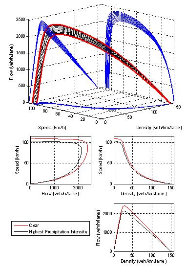
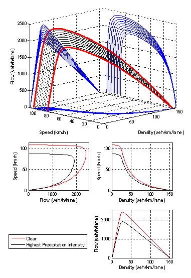
The impact of precipitation intensity on the steady-state speed-flow-density relationship for the Twin Cities data was found to be fairly significant, as illustrated in Figure 5.9. The plot was made for a base case u_f, u_c, q_c, and kj of 110 km/h, 80 km/h, 2,400 veh/h, and 150 veh/km, respectively. The thick 3-D lines depict the base case (upper thick line) and maximum intensity level case (lower thick line). The thin lines represent different intermediate precipitation/visibility levels between the base (no precipitation) case and the maximum (1.50 cm/h precipitation) case. The projection of the 3-D lines on the speed-flow (u-q) plane, flow-density (q-k) plane, and speed-density (u-k) plane is also illustrated in the figure. The figure demonstrates a high-level of variability in the uncongested regime in the speed-flow and speed-density planes with minimum variability in the flow-density plane. In the congested regime a high-level of variability is only observed in the flow-density plane. In addition, the various 2-D plots illustrate the variation in the traffic stream model on each of the three planes. The thick lines represent clear conditions while the thin lines represent traffic stream behavior at the highest precipitation level.

Figure 5.9 Sample Traffic Stream Model Variation
(Twin Cities – Rain)

Similarly, Figure 5.10 illustrates the traffic stream behavior as a result of snow precipitation. A comparison of both figures clearly illustrates the more significant impact snow precipitation has on traffic stream behavior.

Figure 5.10 Sample Traffic Stream Model Variation
(Twin Cities – Snow)

The next step in the analysis was to investigate the potential for regional differences in weather impacts on traffic stream behavior. The regional differences in free-flow speed, speed-at-capacity, and capacity was conducted using a General Linear Model (GLM) instead of an Analysis of Variance (ANOVA) test because the data were not balanced (different number of observations for different city and intensity combinations), as summarized in Table 5.6. The results demonstrated that in the case of rain precipitation the free-flow speed and ratio of speed-at-capacity to free-flow speed were statistically different, as demonstrated in Table 5.7 and Figure 5.11. A Tukey’s comparison demonstrated that these differences occurred between Baltimore and the Twin Cities. Alternatively, differences in the capacity WAFs were not found to be statistically significant. In the case of snow, there was no statistical evidence for differences in the ratio of speed-at-capacity to free-flow-speed, while the free-flow speed and capacity reductions were found to be statistically significant across the various sites, as demonstrated in Table 5.7 and Figure 5.12. Again, this significant difference was only found to occur between Baltimore and the Twin Cities. It is interesting to note here, that the average annual snow precipitation for the Twin Cities was higher than that for Baltimore (7.33 versus 5.57 cm / 2.89 versus 2.19 in). Consequently, one may expect that given the higher annual snow fall rate in the Twin Cities Area, that drivers would be more accustomed to snow and thus would be less impacted by it, however, the results demonstrate the opposite. One interpretation could be that the Twin Cities drivers are more aware of the dangers of driving in snow and thus are more cautious than drivers in the Baltimore Area. However, further analysis is required to investigate the potential causes for these differences in driver behavior.

Table 5.6 General Linear Model (GLM) – Analysis of Variance

Source	D.F.	Seq SS	Adj SS	Adj MS	F	P
City	2	0.0091430	0.0104431	0.0052215	7.35	0.001
Intensity (City)	11	0.0286104	0.0286104	0.0026009	3.66	0.000
Error	125	0.0888420	0.0888420	0.0007107	[no value]	[no value]
Total	138	0.1265954	[no value]	[no value]	[no value]	[no value]

 

Table 5.7 Analysis of Variance Summary of Results

Precipitation Type	Parameter	Factor	P-value
Rain	uf	City	0.001
Rain	uf	Intensity	0.000
Rain	uc/uf	City	0.032
Rain	uc/uf	Intensity	0.025
Rain	qc	City	0.431
Rain	qc	Intensity	0.002
Snow	uf	City	0.000
Snow	uf	Intensity	0.224
Snow	uc/uf	City	0.882
Snow	uc/uf	Intensity	0.816
Snow	qc	City	0.016
Snow	qc	Intensity	0.579

 

Figure 5.11 Variation in Weather Adjustment Factors as a Function of Rain Intensity

[D]

 

Figure 5.12 Variation in Weather Adjustment Factors as a Function of Snow Intensity

[D]

5.2 Conclusions

The research results reported in this section quantified the impact of inclement weather (precipitation and visibility) on traffic stream behavior and key traffic stream parameters, including free-flow speed, speed-at-capacity, capacity, and jam density. The analysis was conducted using weather data (precipitation and visibility) and loop detector data (speed, flow, and occupancy) obtained from Baltimore, Twin Cities, and Seattle in the USA. The study demonstrated the following:

1. Traffic stream jam density is not impacted by weather conditions.
2. Light rain (0.01 cm/h / 0.0039 in/h) results in reductions in the traffic free-flow speed, speed-at-capacity, and capacity in the range of 2 to 3.6 percent, 8 to 10 percent, and 10 to 11 percent, respectively. These results are consistent with the 2 percent free-flow speed reductions for light rain conditions that were reported in earlier studies (Ibrahim and Hall 1994).
3. Reductions in free-flow speed and speed-at-capacity generally increase with rain intensity. The maximum reductions are in the range of 6 to 9 percent and 8 to 14 percent for free-flow speed and speed-at-capacity, respectively at a rain intensity of approximately 1.6 cm/h (0.63 in/h). Earlier studies had shown reductions in free-flow speed in the range of 4.4 to 8.7 percent (Ibrahim and Hall 1994) in heavy rain. Furthermore, the HCM suggests reductions in free-flow speed in the range of 4.8 to 6.4 percent in heavy rain.
4. Roadway capacity reductions remain constant (10 to 11 percent reductions) and are not affected by the rain intensity in the rain intensity range of 0 to 1.7 cm/h (0 to 0.67 in/h).
5. Snow precipitation results in larger reductions in traffic stream free-flow speed and capacity when compared to rain.
6. Light snow (0.01 cm/h) produces reductions in free-flow speed, speed-at-capacity, and capacity in the range of 5 to 16 percent, 5 to 16 percent, and 12 to 20 percent, respectively.
7. Typically reductions in free-flow speed and speed-at-capacity increase with an increase in the snow intensity. The maximum reductions are in the range of 5 to 19 percent at a snow intensity of approximately 0.3 cm/h (0.12 in/h) (intensity measured in equivalent liquid-equivalent precipitation). Ibrahim and Hall had observed reductions in free-flow speed in the range of 33 to 43 percent in a study conducted in Canada.
8. The study demonstrated that the Twin Cities experienced more significant reductions in the traffic stream free-flow speed and speed-at-capacity under snowy conditions when compared to Baltimore (19 versus 5 percent reductions). This finding might appear to be counter intuitive given that the Twin Cities experience higher annual snow precipitation when compared to Baltimore. A possible explanation for this finding is that drivers who are more accustomed to snow are more aware of the dangers of snow. This could also explain the higher reductions that were observed in the Canadian study (33 to 43 percent).
9. Reductions in roadway capacity are not impacted by the snow intensity (range between 12 and 20 percent).
10. Visibility seems to have a larger impact on traffic stream parameters for snow precipitation when compared to rain. Reductions in the range of 10 percent are observed for a reduction in visibility from 4.8 to 0.0 km (3.0 to 0 mi).

Finally, the study also developed free-flow speed, speed-at-capacity, and capacity weather adjustment factors that vary as a function of the precipitation type, precipitation intensity, and visibility level. These factors can be implemented within the HCM freeway procedures.