|
|
|
Travel Time Reliability:
Making It There On Time, All The Time
Overview
Travel time reliability is an increasing concern of travelers, shippers, and businesses. Recent advances in data collection mean that travel time reliability can now be quantified. This report provides guidance in answering the following questions:
- What is travel time reliability?
- Why is travel time reliability important?
- What measures are used to quantify travel time reliability?
- What are the steps for developing travel time reliability measures?
- Case studies illustrating steps to calculate reliability measures?
- Who is using realiability measures?
What is travel time reliability?
Few people will dispute the fact that traffic congestion is common in many cities in the United States. In these cities, drivers are used to congestion and they expect and plan for some delay, particularly during peak driving times. Many drivers either adjust their schedules or budget extra time to allow for traffic delays. But what happens when traffic delays are much worse than expected? Most travelers are less tolerant of unexpected delays because they cause travelers to be late for work or important meetings, miss appointments, or incur extra childcare fees. Shippers that face unexpected delay may lose money and disrupt just-in-time delivery and manufacturing processes.
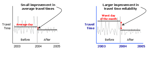
In the past, we have communicated traffic congestion only in terms of simple averages (left side of Figure 1). However, most travelers experience and remember something much different than a simple average throughout a year of commutes (right side of Figure 1). Their travel times vary greatly from day to day, and they remember those few bad days they suffered through unexpected delays.
Figure 1. Averages do not tell the full story
(Click figure to enlarge)
Travel time reliability measures the extent of this unexpected delay. A formal definition for travel time reliability is: the consistency or dependability in travel times, as measured from day-to-day and/or across different times of the day.
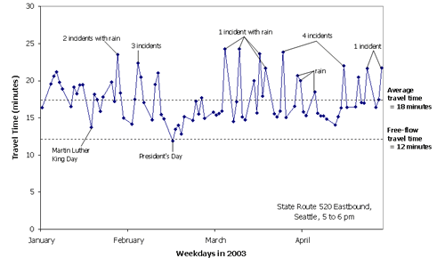
Figure 2 further illustrates travel time reliability with data from a major commuter route in Seattle, Washington. If there is no congestion on this route, travel times are about 12 minutes (e.g., see President's Day in the figure). On all other weekdays, the average travel time was 18 minutes, or an average speed of 40 miles per hour (mph). But when traffic incidents and weather combine to cause unexpected delay, it could take nearly 25 minutes, or 39 percent longer. Commuters who travel this route must plan for this variability if they want to arrive on time—the average just will not do. If they plan their commute based on the average travel time, they will be late half the time and early the other half of the time.
Figure 2. Commuters plan trips based on the worst days, not the average day
(Click figure to enlarge)
Source: Traffic Congestion and Reliability: Trends and Advanced Strategies for Congestion Mitigation, September 1, 2005, available at http://ops.fhwa.dot.gov/congestion_report/.
In other words, commuters have to build in a time cushion or buffer to their trip planning to account for the variability. If they build in a buffer, they will arrive early on some days, which is not necessarily a bad thing, but the extra time is still carved out of their day—time they could be using for other pursuits besides commuting.
Why is travel time reliability important?
Travel time reliability is significant to many transportation system users, whether they are vehicle drivers, transit riders, freight shippers, or even air travelers. Personal and business travelers value reliability because it allows them to make better use of their own time. Shippers and freight carriers require predictable travel times to remain competitive. Reliability is a valuable service that can be provided on privately-financed or privately operated highways. Because reliability is so important for transportation system users, transportation planners and decision-makers should consider travel time reliability a key performance measure.
Traffic professionals recognize the importance of travel time reliability because it better quantifies the benefits of traffic management and operation activities than simple averages. For example, consider a typical before-and-after study that attempts to quantify the benefits of an incident management or ramp metering program. The improvement in average travel time may appear to be modest (left side of Figure 3). However, reliability measures will show a much greater improvement (right side of Figure 3) because they show the effect of improving the worst few days of unexpected delay.
Figure 3. Reliability measures capture the benefits of traffic management
(Click figure to enlarge)
What measures are used to quantify travel time reliability?
The measurement of travel time reliability is an emerging practice; however, a few measures appear to have technical merit and are easily understood by non-technical audiences. Most of these measures compare days with high delay to days with average delay. The four recommended measures: 90th or 95th percentile travel time, buffer index, planning time index, and frequency that congestion exceeds some expected threshold, are explained below.
Perhaps the simplest measure of travel time reliability is 90th or 95th percentile travel times for specific travel routes or trips, which indicates how bad delay will be on the heaviest travel days. The 90th or 95th percentile travel times are reported in minutes and seconds and should be easily understood by commuters familiar with their trips. For this reason, this measure is ideally suited for traveler information. This measure has the disadvantage of not being easily compared across trips, as most trips will have different lengths. It is also difficult to combine route or trip travel times into a subarea or citywide average. Several reliability indices are presented below that enable comparisons or combinations of routes or trips with different lengths.
The buffer index represents the extra buffer time (or time cushion) that most travelers add to their average travel time when planning trips to ensure on-time arrival. This extra time is added to account for any unexpected delay. The buffer index is expressed as a percentage and its value increases as reliability gets worse. For example, a buffer index of 40 percent means that, for a 20-minute average travel time, a traveler should budget an additional 8 minutes (20 minutes × 40 percent = 8 minutes) to ensure on-time arrival most of the time. In this example, the 8 extra minutes is called the buffer time. The buffer index is computed as the difference between the 95th percentile travel time and average travel time, divided by the average travel time.
This formulation of the buffer index uses a 95th percentile travel time to represent a near-worst case travel time. Whether expressed as a percentage or in minutes, it represents the extra time a traveler should allow to arrive on-time for 95 percent of all trips. A simple analogy is that a commuter or driver who uses a 95 percent reliability indicator would be late only one weekday per month.
The planning time index represents the total travel time that should be planned when an adequate buffer time is included. The planning time index differs from the buffer index in that it includes typical delay as well as unexpected delay. Thus, the planning time index compares near-worst case travel time to a travel time in light or free-flow traffic. For example, a planning time index of 1.60 means that, for a 15-minute trip in light traffic, the total time that should be planned for the trip is 24 minutes (15 minutes × 1.60 = 24 minutes). The planning time index is useful because it can be directly compared to the travel time index (a measure of average congestion) on similar numeric scales. The planning time index is computed as the 95th percentile travel time divided by the free-flow travel time.
As with the buffer index, a 95th percentile travel time is used. Other percentiles, such as the 85th, 90th, or even 99th percentile, could be used depending upon the desired level of reliability. For example, a lower percentile may be used in calculating reliability measures for less critical routes or trips.
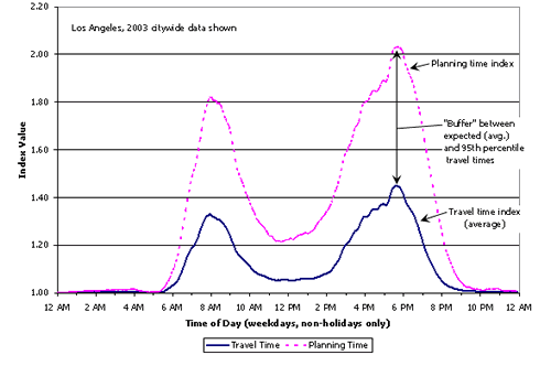
Figure 4 illustrates the relationship between the travel time index, the buffer index, and the planning time index. The travel time index represents the average additional time required during peak times as compared to times of light traffic. The buffer index represents the additional time that is necessary above the average peak travel time, whereas the planning time index represents the total travel time that is necessary.
Figure 4. Reliability measures are related to average congestion measures
(Click figure to enlarge)
Source: Mobility Monitoring Program, http://mobility.tamu.edu/mmp/.
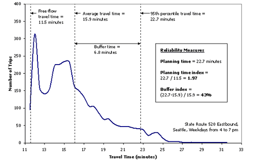
Figure 5 shows a similar relationship in the form of a frequency distribution for trip travel times. The figure shows an example of calculating the average travel time and the size of the "buffer"—the extra time needed by travelers to ensure a high rate of on-time arrival, which helps to illustrate a variety of reliability measures that describe reliability in slightly different ways:
- Planning time – The total travel time, which includes buffer time (i.e., calculated as the 95th percentile travel time).
- Planning time index – How much larger the total travel time is than the ideal or free-flow travel time (i.e., calculated as the ratio of the 95th percentile to the ideal). In the example route shown in Figure 5, the ideal travel time is 11.5 minutes, assuming that vehicles will travel at 60 miles per hour (mph) when no congestion is present.
- Buffer time – The extra time required (i.e., calculated as the difference between the 95th percentile travel time and the average travel time).
- Buffer index – The size of the buffer as a percentage of the average (i.e., calculated as the 95th percentile minus the average, divided by the average).
Figure 5. Reliability measures are easy to calculate with continuous data
(Click figure to enlarge)
Source: Traffic Congestion and Reliability: Trends and Advanced Strategies for Congestion Mitigation, September 1, 2005, available at http://ops.fhwa.dot.gov/congestion_report/.
The last reliability measure presented here is frequency that congestion exceeds some expected threshold. This is typically expressed as the percent of days or time that travel times exceed X minutes or travel speeds fall below Y mph. The frequency of congestion measure is relatively easy to compute if continuous traffic data is available, and it is typically reported for weekdays during peak traffic periods.
Several statistical measures of variability have been suggested to quantify travel time reliability, such as standard deviation and coefficient of variation. These are discouraged as performance measures, as they are not readily understood by non-technical audiences nor easily related to everyday commuting experiences.
What are the steps to develop travel time reliability measures?
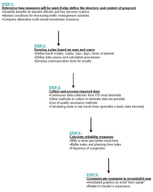
Now that you understand the basics of travel time reliability, you may be asking "How can I start producing travel time reliability statistics in my city?" The steps shown in Figure 6 serve as an outline, with additional technical details, measure calculation procedures, and case study examples provided in the following sections.
Figure 6. A methodical approach can be used to produce travel time reliability measures
(Click figure to enlarge)
Steps to develop travel time reliability measures
Step 1: Determine how the reliability measures will be used
How you plan to use reliability measures will help to define nearly all aspects of measuring and calculating travel time reliability. Thus, this first step is vitally important for defining the structure and content of your program. Typical questions to ask include:
- Will the reliability measures be used to quantify the benefits of existing traffic operations to elected officials? If so, then continuous traffic data will most likely be available to calculate reliability using easy-to-understand measures.
- Will the reliability measures be used to monitor statewide highway travel conditions? If so, "special studies" data collection may be required on roadways where continuous traffic data is not collected for operations purposes.
- Will the measures be used to compare alternative multi-modal investment scenarios in the future? If so, then travel times will have to be estimated using forecasting or simulation models as part of the planning process.
Understanding how the reliability measures will be used and by whom will provide a strong foundation for your performance measurement program. Figure 7 shows an example application of reliability measures for traffic operations. In this example, the reliability measures will be used by upper management and planners to determine baseline levels of travel time reliability (Level 1). Further analysis can identify what is causing unreliable travel (Level 2). Activities, procedures, and policies are then initiated to target specific areas of improvement (Level 3).
Figure 7. Establish who will use reliability measures and how they will use them
(Click figure to enlarge)
Step 2: Develop a plan based upon intended uses and users
Once the intended uses and users have been defined in Step 1, a plan should be developed that outlines various elements related to collecting data, calculating measures, and reporting results (Steps 3 through 5). For example, the plan should cover information such as:
- What travel modes will be included?
- What routes, trips, or roadways will be included?
- What days and time periods are of interest?
- How will data be collected, gathered, or estimated?
- What data processing or reduction steps are necessary once we accumulate the data?
- What reliability measures will be calculated?
- What database or software applications will be used to calculate measures?
- What tables, charts, or graphics will be used to communicate reliability?
- How frequent will reliability be reported?
- How will you get user feedback on the reliability measures?
Step 3: Collect and process required data
Data collection
The basis for all of the reliability measures is route or point-to-point travel times. There are four basic ways in which these travel times can be developed:
- Directly calculated from continuous probe vehicle data;
- Estimated from continuous point-based detector data;
- Collected in periodic special studies (e.g., floating car runs); and,
- Estimated using computer simulation, sketch planning, or demand forecasting models.
The selection of data collection techniques will be based largely on the intended use(s) of the reliability measure, program scope, and available resources. It is possible that more than one of these data collection techniques could be used to obtain travel time data.
Discretion should be used when directly comparing travel times from different methods, as each method may have unique but consistent internal biases. Consider, for example, that travel times along a particular route have been collected for three years using periodic special studies. The deployment of point-based detectors in the fourth year provides the ability to estimate travel times using spot speeds. Caution is advised in making direct comparisons between the first three years of travel time data (from special studies) and the fourth year (from continuous point-based detectors).
Currently, there are few agencies that continuously collect travel time data by direct measurement (such as probe vehicles). It is recognized that all methods of calculating or estimating travel time data produce some error. Professional judgment should be used to determine whether the likely estimation errors exceed those permissible for the applications of the reliability measures. Agencies should also recognize that near-term and future advances in traffic monitoring are likely to provide more than sufficient quantity and quality of travel time data for reliability measures.
Data processing
Once travel time data have been collected or gathered, it is likely that some intermediate data processing or reduction will be necessary. In most cases, the data will be collected or gathered in a more detailed format than is needed for calculation of reliability measures. For example, probe vehicle data will need to be associated with roadway links and combined for specified time periods. Point-based detector data will require the estimation of link-based travel time for aggregate time periods. Travel time data from special studies will need to be downloaded from field collection equipment and integrated into a database. Travel time data estimated from modeling processes will have to be imported into a database.
This step also includes quality assurance to ensure that accurate and valid travel times are used in the calculation steps. Quality assurance may be more significant in this step if the travel time data have been collected for real-time applications but archived for historical use (such as with archived probe vehicle or detector data from traffic operations). The real-time applications may have different quality requirements; thus, additional quality assurance may be necessary. Quality assurance for periodic special studies (such as floating car runs) should be integrated throughout the data collection and reduction process.
Travel time calculation
Once quality assurance has been performed and necessary data processing and reduction has occurred, route travel times should be calculated for the applicable days and time periods. The exact procedures for calculating or estimating travel times from point or link data are not included in this guidance, as many possible methods and variations exist. There are numerous technical resources available that provide detailed information on travel time estimation. Perhaps of most importance are the consistency of estimation methods and the recognition of potential bias errors through sensitivity analyses.
The days and time periods for which travel times are calculated will similarly be defined by determining what conditions the reliability measures are to represent. For example, do you want to represent the reliability of travel for a particular season (several months) or the full year? Individual travel times will be required for those days that are to be represented. Do you want to differentiate the reliability during different times of the day (i.e., "peak of the peak" vs. "shoulders of the peak" vs. off-peak)? If so, individual travel times will be required during these different times of the day.
Step 4: Calculate reliability measures using route/trip travel times
Now that route/trip travel times have been calculated for the days and time periods of interest, we can use some basic equations for calculating the various reliability measures. Three of the four reliability measures require the calculation of a percentile—the frequency of congestion does not require percentiles. Most database or spreadsheet software applications provide a built-in function to calculate percentiles.
Reliability measures:
- 95th or other percentile travel time – calculate directly with database or spreadsheet function
- Buffer index – calculate using Equation 1
- Planning time index – calculate using Equation 2
- Frequency of congestion – calculate by counting the frequency that traffic conditions exceed a preset threshold
Equation 1

Equation 2

Note that these equations are for a specific route/trip and time period. The average planning time or buffer index values (across several road sections, time periods, etc.) can be calculated by using the vehicle-miles of travel (VMT) as a weighting factor (Equation 3).
Equation 3

Step 5: Communicate measures in easy-to-understand tables and graphics
Once reliability measures have been calculated, the results should be displayed in easy-to-understand tables and graphics that meet the needs of your users and uses (Step 1). There are numerous possibilities for communicating travel time reliability measures. Agencies are reminded to consider the likely audiences when communicating reliability measures, as well as to explain the reliability measures in a way that resonates with commuters and travelers. For example, the statistical formulation of 95th percentile is technically meaningful but not easily understood. Instead, use an analogy like "the worst traffic day of the month" (1 of about 20 workdays equals the 95th percentile).
Case Studies Illustrating Steps to Calculate Reliability Measures
Two hypothetical case studies are presented below to illustrate the process of calculating reliability measures. Case Study #1 and Case Study #2 have been simplified, but represent realistic scenarios that are likely to occur.
Case Study #1: Before-and-after evaluation of freeway incident management program
A large urban area is required to evaluate their freeway incident management program, which covers approximately 200 centerline miles of freeway. The evaluation is being performed in response to a request from elected officials and decision-makers to ensure the program is effective. Traffic operations personnel would also like to monitor the effectiveness of the program on a periodic basis.
Step 1: Determine how measures will be used
The evaluation results will be used by elected officials. In addition, traffic operators will use the analysis results to fine-tune incident management procedures as needed. The region has a continuous data source (inductance loop detectors) that provides lane-by-lane volume and speed data, which is archived and available for analysis.
Step 2: Develop a plan based on uses and users
The plan considers the following questions; short answers are provided:
What travel modes will be included?
Auto mode along the general-purpose lanes and transit/auto along the HOV lanes.
What routes, trips, or roadways will be included, and what days and time periods are of interest?
Morning (6 to 9 a.m.) and afternoon (4 to 7 p.m.) peak periods along the seven freeway routes covered by the program. General-purpose and HOV lanes analyzed separately. Analysis sections (3 to 5 miles long) with similar geometry will be identified.
How will data be collected, gathered, or estimated?
Archived inductance loop detector data.
What data processing or reduction steps are necessary?
Quality control of suspicious/incorrect data from the archived data. Expanding point detector speed estimates to morning and afternoon peak period corridor travel time estimates.
What reliability measure(s) will be calculated?
Buffer index.
What database or software applications will be used to calculate measures?
Database software to check for suspicious/incorrect data and to compute corridor travel time estimates.
What tables, charts, or graphics will be used to communicate reliability?
Yearly trends of incident response and clearance times, average travel times, travel time index and buffer index including three years prior to the program and the one year that the program has been in existence. Results broken out by peak period (and direction) and HOV vs. general-purpose lanes. Summary table of results.
How frequently will reliability be reported?
Every six months.
How will user feedback on the reliability measures be obtained?
Solicit feedback from elected officials and operations personnel.
Step 3: Collect and process required data
Archived data are analyzed for the three years before and one year after program implementation. Database software is used for data quality assurance and to aggregate lane-by-lane point detector speeds to section travel times.
Step 4: Calculate reliability measures using route/trip travel times
Compute buffer index (see Equation 1). Corridor travel time index and buffer index values are computed by weighting section values by VMT (see Equation 3).
Step 5: Communicate measures in easy-to-understand tables and graphics
Develop graphics identified in Step 2. Trend analysis graphics can be annotated to indicate how the findings relate to traveler's experiences. In particular, the results can identify the travel time reliability improvement in the HOV lane compared to the general-purpose lanes as well as the added improvement of the incident management program.
Case Study #2: Urban freeway travel time reliability monitoring
A state department of transportation (DOT) would like to monitor urban freeway travel time reliability in a large urban area. Understanding the need to track more than just average travel conditions, the DOT would like to begin monitoring travel time reliability on a quarterly basis. Travel time data are collected continuously through toll tag technology and archived.
Step 1: Determine how measures will be used
The evaluation will be used for internal purposes related to traffic operations. The DOT currently uses numerous traffic management strategies, including surveillance cameras, incident management program, closed-circuit televisions, and ramp meters. Evaluating travel time reliability for specific corridors will assist in identifying specific corridors where the operations treatments may require fine-tuning, while monitoring the entire system will provide an overall assessment.
Step 2: Develop a plan based on uses and users
The plan considers the following questions; short answers are provided:
What travel modes will be included?
Motorists in the general-purpose lanes.
What routes, trips, or roadways will be included and what days and time periods are of interest?
Morning (6 to 9 a.m.) and afternoon (4 to 7 p.m.) peak periods along the entire 300 centerline miles covered by tag readers. Analysis sections will be identified (3 to 5 miles) with similar geometry.
How will data be collected, gathered, or estimated?
Archived toll tag travel time data.
What data processing or reduction steps are necessary?
Quality control of suspicious/incorrect data from the archived data. Computing average sectional travel times for the morning and afternoon peak period.
What reliability measure(s) will be calculated?
Buffer index, planning time index.
What database or software applications will be used to calculate measures?
Database software is used to check for suspicious/incorrect data and to compute peak-period corridor travel time estimates from link and section data.
What tables, charts, or graphics will be used to communicate reliability?
Yearly trends of travel time index, buffer index and planning time index for the past five years of archived data by quarter. Results broken out by facility and peak period (and direction) for the general-purpose lanes. Time-of-day graphics indicating peaking characteristics and comparison between the travel time index and planning time index (see Figure 4). Summary table of results.
How frequently will reliability be reported?
Every three months.
How will user feedback on the reliability measures be obtained?
Solicit feedback from operations personnel.
Step 3: Collect and process required data
Archived data are analyzed for the previous five years. Database software is used for data quality assurance and to aggregate link travel times to section travel times.
Step 4: Calculate reliability measures using route/trip travel times
Compute buffer and planning time index (see Equations 1 and 2). Corridor travel time index, buffer index and planning time index values can be computed by weighting section values by VMT (see Equation 3).
Step 5: Communicate measures in easy-to-understand tables and graphics
Develop graphics identified in Step 2. Trend analysis graphics can be annotated to indicate how the findings relate to traveler's experiences. The graphics can also be annotated for each section/corridor with the extent of operations treatments present. This would assist DOT operations personnel in identifying where unreliable travel conditions exist and the existing operations treatments that might be altered (coverage, timing) to improve reliability.
Who is using reliability measures?
Travel time reliability measures are relatively new in transportation analyses, at least for most public agencies who in the past have only been concerned with average conditions. There are a few "early adopters" of reliability measures, and these agencies have primarily used travel time reliability as a performance measure to supplement measures of average congestion. The rest of this section highlights a few examples of how reliability measures are being used.
National traffic congestion and reliability monitoring
Measuring travel time and reliability in freight-significant corridors
State DOT traveler information and performance measures
Travel time reliability at international border crossings
Southern California Association of Governments (SCAG) goods movement study
National Transportation Operations Coalition (NTOC): performance measure initiative
National traffic congestion and reliability monitoring
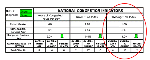
The Federal Highway Administration (FHWA) Office of Operations supports a national traffic monitoring program that incorporates reliability measures. This program tracks reliability measures like the buffer index and planning time index in more than 30 cities. For example, Figure 4 shows the 2003 areawide values for travel time index (average congestion level) and planning time index by time-of-day for Los Angeles. Notice in the chart how, during the peak traffic times, the gap (or buffer) between the planning time index and travel time index increases. This unreliability during peak times means that commuters would have to nearly double their travel time (i.e., planning time index value of 2.0) during light traffic to arrive on-time during rush hour.
One of the ways that FHWA communicates current information on national traffic congestion and travel reliability to key decision-makers is a monthly dashboard report (see Figure 8). This dashboard report includes trend information on the duration (hours of congested travel per day), magnitude (travel time index), and reliability (planning time index).
Figure 8. A reliability measure is included in FHWA's Monthly Congestion Dashboard Report.
(Click figure to enlarge)
Measuring travel time and reliability in freight-significant corridors
FHWA recognizes that the timely and reliable movement of trucks is critical to the economy and a key element of the U.S. DOT's goal to support global connectivity. To better understand how the surface transportation network is accommodating this demand, FHWA launched the Freight Performance Measurement initiative to monitor travel times in freight-significant corridors and delays at major border crossings (http://ops.fhwa.dot.gov/freight/time.htm).
In 2002, FHWA established a partnership with the American Transportation Research Institute (ATRI) to determine whether and how information derived from communications technologies used by the freight industry could provide FHWA with data to support the measurement of freight performance on the surface transportation system. During the initial two phases of the Freight Performance Measurement initiative, ATRI worked with technology vendors and commercial carriers to demonstrate that location data from communications technologies can be used to derive measures of travel time and reliability.
After removing all information except time and location from the Qualcomm satellite data stream, ATRI measured average travel times for five freight-significant corridors—I-5, I-10, I-45, I-65, and I-70. The data were used to derive average travel rates, travel time index and buffer index. Corridor characteristics are shown in Table 1.
From Table 1, applying buffer index data to a freight flow scenario, a commercial vehicle operator moving goods from one end of I-5 (San Diego, CA) to the other end (Blaine, WA) would have to add approximately 6 hours of buffer time ([1,381 miles / 48 mph] x 0.20) to ensure, with 95 percent confidence, that the driver would arrive on time.
Source: Measuring Travel Time in Freight-Significant Corridors, April 2005, available at http://ops.fhwa.dot.gov/freight/time.htm.
State DOT traveler information and performance measures
The Washington State Department of Transportation (WSDOT) quarterly performance report, the Gray Notebook, is one of the nation's leading examples of effective performance monitoring (http://www.wsdot.wa.gov/accountability/). WSDOT continually improves the Gray Notebook to better communicate how it is addressing state transportation issues. In 2002, WSDOT introduced the concept of travel time reliability and recent efforts to distinguish between recurring and nonrecurring congestion. WSDOT acknowledges that travel time reliability is one of the traveling public's most important concerns. WSDOT uses archived freeway operations data to develop several congestion measures (including reliability) for the Seattle region. Examples of the metrics reported by WSDOT include the following, reported as current conditions and changes in annual trends.
- For specific commuter route segments (7 to 24 miles in length):
- The time of day (e.g., 5:20 p.m.) that experiences the worst congestion;
- Travel time on the segment during the peak time;
- "95 percent Reliable Time" (the 95th percentile of travel time);
- Number of days when travel time exceeded twice the free-flow travel time; and
- Percent of days where average route speed was less than 35 mph.
- For entire named freeways in the region:
- Vehicle-hours of delay per day;
- Vehicle-hours of delay per highway mile; and
- Vehicle-miles traveled.
- Case studies documenting before/after congestion conditions.
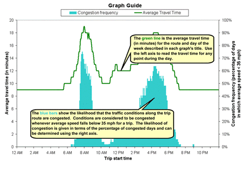
WSDOT provides commuter travel time mobility and reliability information from archived data. Figure 9 illustrates the congestion frequency and average travel time for commuters. Such graphs are available for typical commutes in the Puget Sound area. Travel time reliability is indicated with the congestion frequency, which is the percentage of days in which the average speed is less than 35 mph.
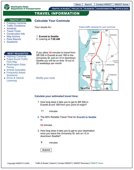
Figure 10 shows another method WSDOT uses to present travel time reliability information to commuters. Commuters can select their particular commute, and the "95 percent Reliable Travel Time" is presented to the user. This value is computed in the same manner as the buffer time described above. In Figure 10, the Internet site indicates that if the commuter allows 59 minutes to travel from Everett to downtown Seattle, they will be on time 19 out of 20 weekdays per month.
Figure 9. WSDOT travel time mobility and reliability corridor data.
(Click figure to enlarge)
Source: WSDOT's Central Puget Sound Average Travel Times web page, available at http://www.wsdot.wa.gov/traffic/seattle/traveltimes/commutes/.
Figure 10. WSDOT commuter reliability information.
Source: WSDOT's Calculate Your Commute web page, available at http://www.wsdot.wa.gov/traffic/seattle/traveltimes/reliability/.
Travel time reliability at international border crossings
The purpose of this FHWA study was to determine a benchmark border crossing delay measure for commercial vehicles (http://www.ops.fhwa.dot.gov/freight/publications/index.htm). Seven ports of entry were surveyed: four on the US/Canada border (Blaine, Ambassador Bridge, Peace Bridge, and Blue Water Bridge) and three on the US/Mexico border (Otay Mesa, El Paso, Laredo). Average delay times were calculated for each port of entry. The delay time represents the difference between the average crossing time and the free-flow crossing time.
A buffer time and buffer index was also calculated for each port of entry. The buffer time is the difference between the 95th percentile crossing time and the average crossing time for all trucks. The buffer time, then, represents the "extra time" above the average that a driver must budget to cross the border and arrive "on time" for 95 percent of the trips. The buffer index is the buffer time expressed as a percentage of average time (i.e., the extra percentage of time that must be budgeted to cross the border). As such, the buffer index eliminates differences in the physical length of crossings and provides a standardized measure among ports.
Table 2 shows the computed operating characteristics for the Ambassador Bridge crossing, including the buffer time and buffer index. Table 2 illustrates that the inbound trip reliability (as measured by the buffer time) is nearly three times as low as the outbound trip.
| Trip | Baseline Crossing Time1 | Average Crossing Time2 | 95th Percentile Time3 | Buffer Time4 | Buffer Index5 |
|---|---|---|---|---|---|
| Outbound | 5.7 | 8.8 | 13.9 | 4.9 | 56% |
| Inbound | 12.9 | 20.4 | 33.9 | 13.4 | 66% |
Notes: 1Baseline time (in minutes) to travel the study distance (between the starting point in the exporting country and the initial inspection point in the importing country) in free-flow traffic conditions. 2Average crossing time (in minutes) to travel the study distance. 3Time (in minutes) for 95 percent of trucks to travel the study distance. 4Time (in minutes) between the average time and the 95th percentile time for trucks to travel the study distance. This is the extra time that must be budgeted to cross the border relative to the average time. 5Buffer time necessary expressed as a percentage of average time. This is the extra percentage of average time that must be budgeted to cross the border. |
|||||
Source: International Border Crossing Truck Travel Time for 2001, April 2002, available at http://www.ops.fhwa.dot.gov/freight/documents/ambass_brdg_over.pdf.
Southern California Association of Governments (SCAG) goods movement study
Substantial growth in harbor freight in the SCAG region is overwhelming surface transportation and reducing air quality and causing noise pollution. SCAG recently completed a study to identify solutions to the issues of goods movement in the SCAG region (http://www.scag.ca.gov/goodsmove/pdf/GoodsmovePaper0905.pdf). SCAG economic staff has been evaluating benefits and costs of increasing transportation logistics infrastructure. Fee structures to support the infrastructure expansion have also been developed by SCAG.
Travel time reliability has been incorporated into the SCAG analysis. The infrastructure proposed (separate truck lanes) would improve travel time reliability for freight movement. SCAG used buffer time to identify the additional time that must be factored into a trip to ensure goods reach their destination on schedule. Table 3 illustrates the results of a 2030 model to estimate the impact on time and reliability with separate truck lanes. The model compared conditions to planned projects being developed. In 2030, a shipper would save 128 actual minutes and another 276 "buffer" minutes for a total of 405 fewer minutes (6.75 hours) for a shipment. This equates to total speed and reliability savings of nearly $500 per trip.
Source: Goods Movement in Southern California: The Challenge, The Opportunity, and The Solution, September 2005, http://www.scag.ca.gov/goodsmove/pdf/GoodsmovePaper0905.pdf.
National Transportation Operations Coalition (NTOC): Performance measure initiative
The NTOC Action Team on Performance Measurement recently conducted an initiative with the goal to define a candidate list of measures commonly agreed upon by federal, state, and local transportation officials (http://www.ntoctalks.com/ntoc/ntoc_final_report.pdf). The initiative included a literature review, electronic survey and discussions by the NTOC team and oversight committee. The process used to identify the measures was designed to ensure the measures were identified and elected by stakeholders who will collect the data, report results, and benefit from learning from best practices. A "one-pager" of each measure was produced that includes the measure definition, what it includes, units of measurement, processing (how to measure), typical applications, short examples, and additional notes (if applicable). Travel time reliability was identified as one of the measures identified by the NTOC team. Specifically, buffer time was identified as the measure and a "one-pager" was created to simply illustrate how the buffer time is computed. Instruction is also provided regarding computation of the measure as an index (percentage).
For additional information
Contact Rich Taylor, FHWA Office of Operations, Rich.Taylor@fhwa.dot.gov, (202) 366-1327.
Produced by Texas Transportation Institute with Cambridge Systematics, Inc., December 2005.
To view PDF files, you need the Adobe Acrobat Reader.

