Chapter 4. Wyoming Interstate 80 Testbed Case Study
This chapter describes development and application of a customized analysis, modeling, and simulation (AMS) tool for evaluating three selected connected vehicle (CV) weather-responsive management strategies (WRMS) applications: traveler information messages (TIM), CV-based variable speed limit (VSL), and snowplow pre-positioning.
Testbed Review
Interstate–80 (I–80) runs 402 miles along the southern edge of Wyoming. It is an east-west connector for freight and passenger travel in the country, as shown in figure 2. The corridor averages more than 32 million tons of freight per year (at 16 tons per truck). The truck volume is 30–55 percent of the total annual traffic stream and comprises as much as 70 percent of the seasonal traffic stream. Several crashes, affecting both commercial and private vehicles, have occurred along I–80 in Wyoming that resulted in fatalities, extended closures, and economic loss. To improve driver safety along the corridor, the Wyoming connected vehicle pilot (CVP) uses dedicated short-range communication-based (DSRC) applications that leverage vehicle-to-vehicle (V2V) and vehicle-to-infrastructure (V2I) connectivity to support advisories, roadside alerts, and dynamic travel guidance for freight and passenger travel.
The test network in this case study is a portion of the Wyoming CVP corridor on I–80 between Cheyenne and Laramie (mileposts 317–340). The total length of the test network is about 23 miles in each direction. V2V and V2I applications will enable communication with drivers for alerts and advisories regarding various road and weather conditions. Information from the V2V and V2I applications is made available directly to vehicles equipped to receive the messages, or through the Wyoming Department of Transportation’s (WYDOT) existing traveler information sources.
In the CVP, WYDOT uses V2V, V2I, and infrastructure-to-vehicle (I2V) connectivity to improve monitoring and reporting of road conditions to and from vehicles on I–80. Five CV applications have been highlighted: forward collision warning (FCW), I2V situational awareness, work zone warning, spot weather impact warning (SWIW), and distress notification (DN).
The Wyoming CVP has deployed significant CV and road weather resources to demonstrate CV applications, including spot weather warnings of potentially hazardous travel conditions. Wyoming already uses information from its snowplow vehicles as input to its VSL analysis process and VSL deployment along sections of I–80. It provided an exceptionally functional testbed for the corridor-specific traffic management strategies investigated in this study. An AMS model built for the safety assessment of the CVP applications provided a basis for the integration of the offline and real-time operations of AMS tools.
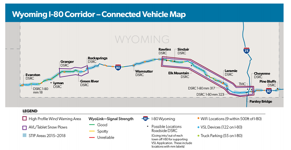
AVL = automated vehicle location. DSRC = dedicated short-range communications.
mm = mile marker. STIP = State Transportation Improvement Plan. VSL = variable speed limit.
Source: Wyoming Department of Transportation
Figure 2. Map. Wyoming Interstate 80 corridor — connected vehicle pilot map.
Locations with dedicated short-range communications are plotted along the highway. These, from east to west are Pine Bluffs, Cheyenne, mile marker 323, mile marker 317, Laramie, Elk Mountain, Sinclair, Rawlins, Wamsutter, Rock Springs, Green River, Granger, Lyman, mile marker 18, and Evanston. Points along the highway are plotted: WiFi locations, where 9 are within 500 feet of the Interstate; 122 variable speed limit locations; and 55 truck parking locations. A high profile wind warning zone is highlighted between Cheyenne and Rawlins. Automated vehicle, tablet snow plow zones are highlighted between Cheyenne and Rawlins and from Rock Springs to Granger. State Transportation Improvement Plan zones are highlighted over most of the map, except for the area between Wamsutter and just east of Rock Springs. WyoLink signal strength is indicated as good, spotty, or unreliable along the Interstate. Zones indicated as good are mostly between Laramie and Rawlins. Spotty and Unreliable locations are not plotted.
Weather-Responsive Management Strategies
This case study evaluated three WRMS, which included two traffic management strategies (TIMs and CV-based VSL) and one winter maintenance strategy (snowplow pre-positioning). The three WRMS were identified as the most beneficial to the testbed corridor, and of the most interest to WYDOT. The CV applications in the CVP, which are all enabled by CV TIMs, are of interest to this project from the traveler information perspective (e.g., real-time information on crashes or work zones). VSL can be communicated through TIMs or on VSL signs that have been installed along I–80. Any CV data related to weather conditions can be used to support the VSL decision-making. Snowplow pre-positioning not only can help clear the road to reduce safety risks, but also provide additional real-time weather data back to the traffic management center or traffic management system (TMC), benefiting other WRMS.
Traveler Information Messages
Traveler information is designed to enable advisory message broadcasting to the vehicle driver based on location and relevant situations. Messages are prioritized, both for delivery and presentation, according to the type of the advisory. Message presentation may be text, graphics, or audio cues. Examples include traveler advisories (traffic information, traffic incidents, major events, evacuations, etc.) and road signs. In this case study, the TIM system is applied in the form of a CV-based weather-responsive application. The TMC delivers the message through the CV roadside unit (RSU) to onboard units (OBU) installed on CVs. The in-vehicle applications parse TIMs from the infrastructure and combine them with vehicle-specific parameters to warn the drivers, if appropriate.
In this case study, TIMs are designed to include necessary information, such as vehicle status, weather parameters, event (e.g., work zone, crashes) information, and static speed limits/VSLs. Therefore, TIMs simulated in this case study can technically enable all of the following five applications in the Wyoming CV testbed. TIM transmission is realized through V2I and V2V communications. Four RSUs are distributed along the corridor, according to the WYDOT Connected Vehicle Monitor (CVM).
Connected Vehicle-Based Variable Speed Limit
Compared with the sign-based VSL, the connected vehicle-based variable speed limit (CV–VSL) provides more options for CV drivers to access VSL information apart from reading VSL signs.(52) In the Wyoming CV testbed, the CV–VSL aims to provide commercial truck drivers with real-time regulatory and advisory speed limits to help them better manage driving speeds under adverse weather conditions and reduce potential speed variances that may cause crashes. Through I2V communication (e.g., DSRC or satellites(53)), drivers can be immediately informed of the dynamic speed limits through in-vehicle devices. For the Wyoming testbed, Yang(54) conducted a driving simulator study to assess the impact of the Wyoming CV–VSL application on truck drivers’ behavior under adverse weather conditions. Simulation results showed that when the advisory speed limits were lower than 55 miles per hour (mph), participants generally followed the VSLs displayed on the CV human-machine interface (HMI).(55) Additionally, traffic flows utilizing CV–VSL technology tend to exhibit lower average speeds and speed variances compared with baseline scenarios, indicating a level of influence of CV behavior on the non-CV behavior. These effects of CV–VSL warnings can potentially bring safety benefits (i.e., reduced average speeds and speed variances, and therefore, reduced risk of crashes) under adverse weather conditions. The influence of CV behavior on non-CV traffic (i.e., smoothing the following traffic, and therefore, reducing speed differences in the traffic stream) is also reported in other studies.(56,57) This implies that even under relatively low market penetration, slowing down a certain portion of vehicles can effectively impact a larger number of vehicles in a traffic stream positively.
Snowplow Pre-positioning
During winter months, snow and ice control is a priority for snow-State departments of transportation (DOT) (e.g., I–80 corridor in this case study). The safety of the traveling public, response times of emergency services, and ongoing access to goods and services all depend on the effectiveness of winter maintenance operations. Routing and positioning of snowplow trucks along the freeways include a variety of decisions. The snowplow pre-positioning strategy optimizes the routes of a fleet of snowplow vehicles, subject to roadway entry and exit constraints. This strategy aims to find the optimal locations for snowplow positions before the weather events, for two purposes: (1) clearing the road to improve roadway conditions and (2) providing additional CV data on weather and other events through weather sensors on the snowplow trucks for TMCs to implement optimal strategies.
In this case study, snowplow pre-positioning is the process of creating a set of snow and ice control routes through pre-positioning to minimize the cost of snow and ice control operations and maximize the safety and mobility performance of the traffic system. Well-designed snowplow pre-positioning strategies can result in more effective and more cost efficient snow and ice control services, because roads are cleared more rapidly. Since the route length remains the same in the test network, costs may be measured in terms of operation times (i.e., the required times to clear the roads), safety, and mobility performance.
Simulation Network Calibration
Simulation modeling of a segment of Wyoming I–80 CVP corridor has been completed as part of the Wyoming CVP, and has been accessed by the research team. The study network is a portion of the Wyoming CVP corridor on I–80 between Cheyenne and Laramie (mileposts 317–340) developed as a VSL. The corridor presents challenging traffic situations, such as high altitude, high adverse weather events, and steep vertical curves.(51)
PTV Group has multiresolution traffic modeling platforms that include macroscopic, mesoscopic, microscopic, and hybrid mesoscopic-microscopic modeling engines.52 The microscopic simulator PTV Vissim was used for the I–80 testbed. The research team considered the microscopic tool as the optimal option for the safety analysis in the I–80 case study. In this analysis, traffic congestion (and related performance measures, such as delay) was not of concern. The testbed focused on safety analysis and the effectiveness of the three selected WRMS in reducing crashes or safety risks. The evaluation of safety risks required detailed individual vehicle space-time trajectories at the subsecond level, which could have only been generated through microscopic simulation tools.
The Vissim model, built for the Cheyenne-Laramie VSL corridor, provides the foundation for the WRMS analysis. The basic corridor network was uploaded from the standard map data in Vissim. The roadway geometric data, including the number of lanes, roadway segment lengths, and grades; the location of lane additions and drops; and locations of rest areas and parking areas have been manually coded in Vissim. The comparison between the specific real-world network and the Vissim model is shown in figure 3. Additional detailed traffic control parameters have been incorporated into the Vissim network to better reflect existing operational conditions. Key traffic parameters include traffic composition, vehicle dynamics data, posted speed limits, and the presence of work zones (including location, length, lane-closure condition, etc.), among others. The car-following behaviors in Vissim under different weather scenarios were also taken into consideration.(51) Calibration and validation results of basic Vissim driver behavior model parameters in response to normal or adverse weather conditions are documented in Gopalakrishna et al.(53) and those are adopted directly in this study. Driver behavior in response to CV applications under investigation are modeled separately in this study and detailed in this chapter.
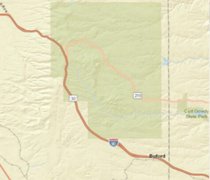
Source: Wyoming Department of Transportation
A. Map. Real-world road segment.
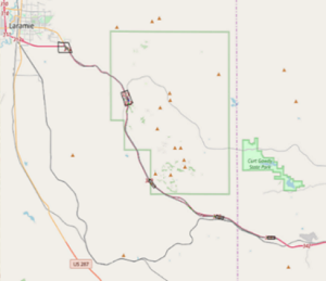
Source: FHWA
B. Map. Vissim simulation road segment.
Figure 3. Maps. Comparison between the real-world and the Vissim network of Interstate 80, Wyoming connected vehicle pilot corridor.
Simulation Framework
A recent Federal Highway Administration (FHWA) Saxton Transportation Operations Laboratory (STOL) and University of California, Los Angeles (UCLA) platform development project using Vissim developed customized functions for CV and weather features. The tool has been used for CV/automated vehicle (AV) applications in multiple ongoing and previous FHWA efforts. To implement various CV applications, three major modules are needed in the AMS tool: the Vissim Network module, the Simulation Manager module, and the application programming interface (API) module. The detailed simulation framework, shown in figure 4, is explained below:
- Vissim Network is the underlying transportation network used for testing a large variety of CV algorithms. In this study, various Vissim networks must be constructed for different weather conditions, as reflected by various types of driver behavior.
- Simulation Manager is enabled through a component object model (COM) interface to support easy scenario building and system-level control. The Simulation Manager allows users to adjust control parameter values crucial for the implementation of CV applications in Vissim without directly accessing the Vissim driver model API source code. It also provides users with an interface to modify simulation scenario parameters, such as market penetration rates (MPR), traffic volumes, and simulation times. The Simulation Manager can be used to realize online or offline implementations of the AMS tool.
- The API module is a program that determines driving behavior by customized programs for corresponding parameters in different CV applications. Vissim is capable of not only conducting conventional simulations of transportation behavior in a network, but also implementing its external driver model through a dynamic linked library (DLL) interface. This substitutes the built-in Vissim driving behavior with a fully user-defined behavior for vehicles. In a proper framework, Vissim passes the current state of a vehicle and its surrounding traffic to the DLL, the DLL computes and determines the succeeding behavior of the vehicle as specified by an algorithm, and the DLL passes the updated state of the vehicle back to Vissim for the next simulation step. This feature allows the user to model (and test) various CV applications.
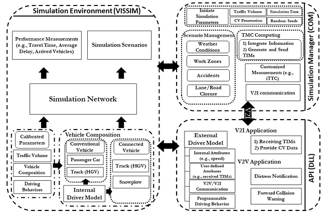
API = application programming interface. COM = component object model. CV = connected vehicle. DLL = dynamic linked library. HGV = heavy-goods vehicle. iTTC = inverse time-to-collision. TIM = traveler information message. TMC = traffic management center. V2I = vehicle-to-infrastructure. V2V = vehicle-to-vehicle.
Source: FHWA
Figure 4. Diagram. Detailed simulation framework of Vissim® network, component object model, and application programming interface.
Performance Measures
The main goal of the I–80 WRMS implementation is to enhance safety performance. While many surrogate safety measures have been proposed and adopted in the literature, in this case study, inverse time-to-collision (iTTC) is applied, as shown in figure 5, to measure longitudinal collision risks. Time-to-collision (TTC) is defined as the expected time for two vehicles to collide if they remain at their present speed and on the same path. We use iTTC to avoid infinity in numerical computation. Large iTTC values indicate large safety risks. iTTCs smaller than or equal to 0 imply no collision risk, and therefore will not be used in the summation calculations in figure 5.
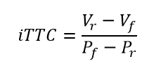
Figure 5. Equation. Calculation of inverse time-to-collision (iTTC).
inverse time-to-collision equals the values of current speed of the following vehicle in meters per second minus current speed of the preceding vehicle in meters per second divided by the value of position of the preceding vehicle in meters minus position of the following vehicle in meters.
Where,
Pf = position of the preceding vehicle (m).
Pr = position of the following vehicle (m).
Vr = current speed of the following vehicle (m/s).
Vf = current speed of the preceding vehicle (m/s).
However, the total iTTC usually does not reflect the real collision risk of a vehicle during the trip in the network, since the longer time a vehicle drives, the higher the total iTTC would be. Thus, iTTC for a group of vehicles, we use the time-weighted iTTC to reflect the average collision risk of all vehicles in the group and avoid the impact of the travel time of each single vehicle. This measurement uses the travel time of each vehicle as a weight to average each vehicle’s unit iTTC in the network.
While the iTTC can serve as a good measure of the overall collision risks in the system, the aggregated values do not distinguish small collision risks with high or extremely high collision risks, which are more likely to cause actual crashes. Therefore, in this case study, the collision risks are further categorized into four levels by iTTC: small risk (0 < iTTC < 0.1 s-1), medium risk (0.1 s-1 < iTTC < 0.2 s-1), high risk (0.2 s-1 < iTTC < 0.3 s-1), and extreme risk (iTTC > 0.3 s-1). Within each risk level, the iTTC is divided into finer intervals with a resolution of 0.02 s-1.
Several strategies in this report (e.g., VSL) improve safety performance by reducing vehicle speed in specific situations. Some research(59) proposed the negative mobility impact of this kind of strategy. While the primary performance optimization of the Wyoming CVP corridor is safety performance, it is also necessary to ensure that mobility efficiency is not significantly compromised. In this case, the average travel time is used to quantify mobility efficiency in order to provide a trade-off between safety and mobility.
Analysis, Modeling, and Simulation for Traveler Information Messages
The simulation of TIM applications in this case study can be generally divided into two sections. The first is TIM data transmission, and the second is how drivers would react to the TIM messages. The data transmission includes both I2V and V2V communications. In this case study, with the use of an API, all CVs in the network calculate the distance between itself and the nearest front vehicle either in the current or adjacent lane at every simulation time step. If a nearby vehicle is a CV and the distance is within the DSRC range (i.e., 300 meters [m] in this case study), the V2V communication module will be activated to allow the TIM message to be transmitted between the two CVs.
Road events included in the above-mentioned applications (e.g., crashes, work zones, spot weather) can lead to a temporary or long-lasting lane closure. All these cases could be included in TIM and delivered to CVs on the roadway. The simulation also needs to handle how drivers would react to the in-vehicle TIM advisories or warnings. In this case study, two applications enabled by TIMs are selected (i.e., early lane-change [ELC] advisory and FCW) to investigate the impact of TIMs on driver behavior and, subsequently, system performance. The ELC advisory and FCW applications are selected because they cause changes in choices of longitudinal acceleration/deceleration and lateral lane selection.
Early Lane-Change Advisory
When a vehicle approaches an event location on the same lane, it may run into slow or braking non-CVs or static objects at the event scene, particularly in low-visibility conditions, resulting in substantial safety risks. Therefore, it is beneficial to let the vehicle make a lane change when possible (i.e., no vehicles blocking the lane change on the adjacent lanes) in order to reduce rear-end crash risks. This ELC advisory message can be included as a part of the TIMs and delivered to each CV. The OBUs can then broadcast this message to the drivers (e.g., via auditory messages).
To model the details of this process, the lane-change behavior is controlled by lane-change desire. The lane-change desire is linearly determined by lane-change distance, defined as the distance from the vehicle to the lane-closure zone. The smaller the distance, the higher the lane-change desire will be. The upper and lower bounds of the lane-change distance are defined as maximum lane-change distance and minimum lane-change distance, separately. The maximum lane-change distance is set as the DSRC communication range. The minimum lane-change distance is a threshold distance that, once lower than this value, the vehicle will be facing high crash risks and will immediately make a lane change. This threshold is set to 100 m in this case study.
In order to ensure the lane-change timing is randomly determined for each vehicle, a random number between zero and one is introduced and used to compare with lane-change desire to simulate the ELC behavior. Once the vehicle enters the ELC section, a random number will be generated and refreshed every simulation time step. The random number is compared with the lane-change desire at every time step. If the lane-change desire is equal to or greater than the random number, the vehicle starts lane changing; if the lane-change desire is less than the random number, the vehicle keeps driving on its current lane. The total ELC logic is shown in figure 6.
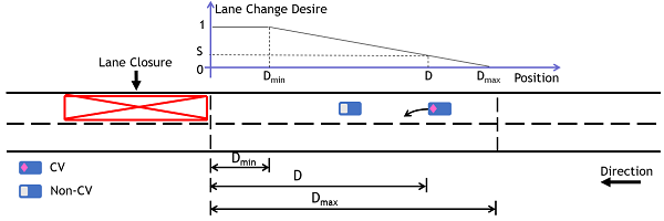
CV = connected vehicle. D = distance. max = maximum. min = minimum.
Source: FHWA
Figure 6. Illustration. Early lane-change logic.
Forward Collision Warning
FCW systems provide visual, audible, or tactile alerts to warn a driver of an impending collision with a car or object in its direct forward path. The warning message can be included as a part of the TIM message and broadcast to drivers via DSRC and OBUs.
Under adverse weather conditions (e.g., heavy fog, snow), visibility distance is insufficient for drivers to promptly react to avoid crashes. FCW relies on I2V and V2V communications to obtain data of the front vehicle and calculate the headway and speed difference. During severe weather conditions, the communication distance is always longer than the sight distance, and therefore, CVs could receive the alert of the forward collision risk before drivers observe the front vehicle.
While FCW can also rely on vehicle sensors, such as vehicle front radar, this case study focuses on CV/DSRC-enabled FCW. That said, if at least one of the two consecutive vehicles is non-CV, the FCW function will not be activated. The front and rear vehicles must all have communication capability and be in the communication range of each other.
In this case study, FCW is categorized into two notification levels: cautionary level (yellow) when iTTC is between 0.2 s-1 and 0.1 s-1, and alert level (red) when iTTC is more than 0.2 s-1. In the cautionary level, there is still enough time for drivers to slow down with a reasonable deceleration. However, if the alert level occurs, the FCW system will provide decision-making to help drivers choose between changing their lanes (to the left or right, if there are multiple lanes) and applying the brake heavily. This decision is determined based on the condition on adjacent lanes.
Except for the lane-change decision, another parameter to be calibrated is driver deceleration choice after receiving the collision warning.(58) If the warning is at the alert level, the deceleration and lane-change behavior are determined by the Vissim default car-following and lane-change models because the drivers need to brake heavily or change lanes to avoid crashes. Vissim can generate reasonable behavior values under this condition. If at the cautionary level, the deceleration may not be directly affected by the front object, and cannot be accurately captured through Vissim’s models. Therefore, the behavior is calibrated using a behavior data set collected by the University of Wyoming of a truck driving simulator with 25 professional truck drivers under adverse weather conditions.(54) The average deceleration under the cautionary level in this experiment is 1.31 feet per second squared (ft/s²) (0.4 meters per second squared [m/s²]). It is regarded as the constant deceleration in this case study when drivers receive cautionary level warnings.
Analysis, Modeling, and Simulation for Connected Vehicle-Based Variable Speed Limit
In this case study, the speed limit information displayed on VSL signs can only be received by vehicles in the visual range. This range is the visibility of drivers under specific weather conditions. This presents spatiotemporal constraints to drivers to receive the information. CVs can also receive speed limit information via the HMI equipped on the vehicles. It is also possible to send this information through satellite or cellular technologies, since VSL is not time-sensitive information and some delay in VSL communication is tolerable, from the perspective of system safety and efficiency. Sending through the satellites will enable communication of dynamic speed limits to all CV drivers in a short time period to achieve more substantial system benefits.
In the former scenario of DSRC communication, the VSL information can only be transmitted from RSUs to CVs. In this situation, only CVs in the RSU communication range can receive the VSL information after the TMC sends the speed limit value information to RSUs. Connected vehicle-variable speed limit (CV-VSL) communicated through DSRC is similar to signed-based VSL, in that it can only inform drivers/vehicles passing the location of the RSUs or signs. The VSL information is included as a part of the TIM. Additionally, the VSL information can be sent through non-DSRC communication channels (i.e., satellite and cellular communication), which can enable immediate notification of dynamic speed limits to all CVs and, therefore, further improve system safety performance. The VSL information is not time sensitive and can be sent through these additional channels, subject to information delay and packet drops, in exchange for systemwide information dissemination. The Wyoming CV testbed also proposes to use satellite communication for this purpose,(53) as illustrated in figure 7. In this scenario, all CVs on the road can receive the VSL information after the TMC broadcasts the speed limit information. Meanwhile, non-CVs can continue to receive the VSL information from roadside signs. It is expected that the systemwide information dissemination can significantly enhance safety performance, and therefore this dissemination approach is targeted in this case study.
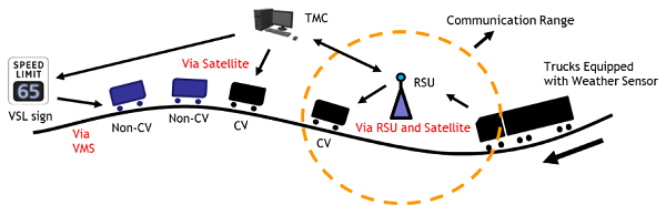
CV = connected vehicle. RSU = roadside unit. TMC = traffic management center. VMS = variable message sign. VSL = variable speed limit.
Source: FHWA
Figure 7. Illustration. Connected vehicle-variable speed limit system using satellite communication.
This illustration is a horizontal view of a roadway so the road is represented as a single solid line extending from right to left. A number of vehicles are represented along the road: trucks equipped with weather sensor, connected vehicles, and non-connected vehicles. A roadside unit tower is drawn above the road, with a dotted yellow circle drawn around the tower that represents the communication range of the unit. The illustration also shows a representation of a traffic management center and a variable speed limit sign. Communication arrows are drawn: from the weather sensor equipped truck to the roadside unit; from the roadside unit to one of the connected vehicles; back and forth between the roadside unit and the traffic management center; from the traffic management center to one of the connected vehicles, via satellite; from the traffic management center to the variable speed limit sign; and from the variable speed limit sign to the roadway variable message sign.
In this case study, we use the same weather-responsive VSL decision strategies that are currently adopted in the Cheyenne TMC.(53) This road weather information system (RWIS) algorithm takes data from RWIS and field staff reports as inputs, and automatically calculates suggested speed limits under specific weather and road conditions. Key weather parameters included in the algorithm are road surface status, humidity, average wind speed, and visibility.
In microscopic traffic simulation, weather and road conditions are reflected using different driver behavioral models through the parameters such as look-ahead distance, desired following gap, and desired velocity. These parameters are frequently associated with roadway links of the simulation network, such that specific weather and road conditions can be reflected through driving behavior for different parts of the freeway. By referring to these parameters, a mapping between RWIS weather data and weather-sensitive driving behavior parameters was created in this case study. The AMS tool first receives data on weather and road conditions, and the mapping determines the specific set of driving behavior parameters to use in the simulation evaluation. In the meantime, the Cheyenne TMC algorithm is used to determine the speed limits and directly implemented in the simulation. An example mapping is shown in chapter 5 to enable the simulation evaluation for this case study.
Analysis, Modeling, and Simulation for Snowplow Pre-Positioning
The snowplow pre-positioning strategy refers to deployment of snowplow trucks at key roadway segments ahead of severe weather events, such that accumulated snow on the road can be cleared as early as possible. This has two positive effects on traffic safety: (1) clearing the road to improve roadway conditions and (2) providing additional real-time weather and road condition data to the TMC.
According to the Wyoming CVP, there are approximately 60 total snowplow trucks deployed along the 403-mile I–80 corridor. It is assumed that the number of snowplows that serves in this 23-mile segment for simulation can be proportionally scaled down by distance to four.
The application of snowplow pre-positioning aims to optimize the deployment strategy of snowplows. With the snowplow pre-positioning strategies applied, the roadway surface is expected to be improved so that the overall safety performance could be enhanced more quickly. Meanwhile, the operation of plowing should be completed as soon as possible, and the snowplow operations should cause the least amount of interruptions to the traffic.
Improving roadway conditions can be simulated in Vissim by changing the vehicle’s car-following behavioral parameters. In Vissim, maximum and minimum accelerations are attributes of the link driving behaviors, and this behavior is associated with roadway links as an attribute of the links. In this case study, it is assumed that a link will be plowed by two snowplow trucks before the snowplowing job is completed for the link, and the corresponding driving behavior parameter set for better road and weather conditions will be used after the plowing is completed. This is considered reasonable because the driving condition can be much improved by the snowplow. However, it will require an additional calibrated parameter set to reflect this driving condition after the link is plowed. Since no such data are available to the research team, the parameter set of clear weather condition was used as a rough surrogate. Similarly, Vissim does not contain modules that directly simulate the road surface condition. To simulate the influence snowplows have on the surface, and their impact on traffic safety performance, different link driving behavior types are applied for the same roadway to represent the surface condition before and after plowing. All snowplow trucks drive at a relatively low speed while plowing the road (25 mph). Once a link is twice passed by snowplows, it is defined as a plowed link.
Because the route length remains the same (23 miles), the consideration becomes how to group the snowplows and where to pre-position them to achieve optimal system performance, in terms of safety and mobility. Because this test network is only a segment of the CV corridor, and the plowing operations may be conducted jointly with adjacent segments, the actual plowing strategies can be different from those discussed in this study. However, the focus here is to understand how two realistic pre-positioning strategies can improve system safety and what the magnitude of safety enhancements is. The base case and pre-positioning cases evaluated in this study are defined as follows:
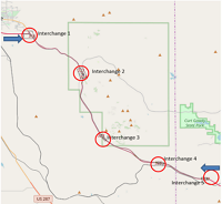
- Base case (single-point positioning): in the base case, all snowplows enter the network from one end of the freeway segment, as shown in figure 8A.
- Pre-positioning case 1 (two-point positioning): four snowplow trucks are divided into two groups, and each group contains two trucks. The two groups of snowplows start plowing simultaneously from the end of the eastbound and the end of the westbound freeway segment (i.e., Interchanges 1 and 5 in figure 8B).
- Pre-positioning case 2 (multipoint positioning): four snowplow trucks are divided into four groups, and each contains only one snowplow. The snowplow trucks enter the network from Interchanges 1, 3, and 5 and start plowing simultaneously, as shown in figure 8C.
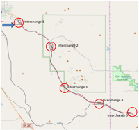
A. Map. Base case.
Map shows Interstate 80 between Cheyenne and Laramie. Circles are drawn indicating locations of five interchanges at regular intervals along the highway: interchange 1 at Laramie, and interchange 5 at Cheyenne. Interchanges 2, 3, and 4, are about equally spaced between 1 and 5. Map A is labeled base case and shows a blue arrow at interchange 1.
B. Map. Case 1.
Map shows Interstate 80 between Cheyenne and Laramie. Circles are drawn indicating locations of five interchanges at regular intervals along the highway: interchange 1 at Laramie, and interchange 5 at Cheyenne. Interchanges 2, 3, and 4, are about equally spaced between 1 and 5. Map B is labeled case one and shows blue arrows at interchanges 1 and 5.
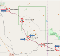
C. Map. Case 2.
Map shows Interstate 80 between Cheyenne and Laramie. Circles are drawn indicating locations of five interchanges at regular intervals along the highway: interchange 1 at Laramie, and interchange 5 at Cheyenne. Interchanges 2, 3, and 4, are about equally spaced between 1 and 5. Map C is labeled case two and shows a single blue arrow at interchange 1, two blue arrows at interchange 3, and a single blue arrow at interchange 5.
Original maps: © Google® Maps™. Map overlays: FHWA (see Acknowledgments).
Figure 8. Maps. Three snowplow pre-positioning scenarios.
System Parameters
In the Vissim network calibrated as a part of the Wyoming CVP, three weather scenarios are designed: normal/clear, snowy, and severe weather conditions. These scenarios can clearly distinguish between different weather conditions, pavement conditions, and visibility levels. Therefore, they are representative of varying weather conditions of I–80 during winter seasons. As previously indicated, three CV-based WRMS are introduced and evaluated for the I–80 study: TIM, VSL, and snowplow pre-positioning. The driver behavior differences under the three weather scenarios are in terms of speed distribution, look-ahead distances, and other behavioral parameters. For driving behavior, apart from some basic parameters such as visibility and look-back distance, Vissim’s Wiedemann 99 model parameters (CC0–CC9) are calibrated, as shown in table 6.
Table 6. Car-following parameters used for clear, snowy, and severe weather in this study.
| W99 Model Parameters |
Clear |
Snowy |
Severe |
| CC0: standstill distance (m) |
4.2 |
3.05 |
6.1 |
| CC1: spacing time (s) |
0.7 |
0.9 |
0.9 |
| CC2: following variation, max drift (m) |
12.7 |
16.1 |
6.1 |
| CC3: threshold for entering following (s) |
-24.6 |
-8 |
-8 |
| CC4: negative following threshold (m/s) |
0.0 |
-0.35 |
-0.35 |
| CC5: positive following threshold (m/s) |
0.9 |
0.35 |
0.35 |
| CC6: speed dependency of oscillation (10-4 rad/s²) |
1.7 |
11.4 |
11.4 |
| CC7: oscillation acceleration (m/s²) |
1.0 |
0.25 |
0.25 |
| CC8: standstill acceleration (m/s²) |
1.4 |
3.5 |
3.5 |
| CC9: acceleration at 80 km/h (m/s²) |
0.1 |
1.5 |
0.91 |
Different CV MPRs are considered to understand the system performance sensitivity with varying percentages of CVs in the system. In this study, the CV MPR is defined as the proportion of CVs in all heavy-goods vehicles (HGV) (i.e., trucks). HGVs are the focus of the I–80 CV testbed, which aims to equip trucks with DSRC capabilities to enhance their operational safety. The CV MPRs of HGVs include 0 percent, 20 percent, 40 percent, 60 percent, 80 percent, and 100 percent. To eliminate the confounding effects caused by the traffic volume, traffic volume in all scenarios are set at the same level as in the severe weather conditions. The total simulation time is 7,800 seconds, including a 600-second warm-up period. For each scenario, results from five simulations using random seeds are averaged to account for the randomness in simulation.
To create external conditions on the network, four active lane-closure events (e.g., work zones, incidents, crashes) are used, including two for the eastbound and two for the westbound. In each of the four events, the right-most lane is closed for 646.17 feet (200 m), leaving the left-most lane open for vehicles to bypass the events. Each event starts and ends at different simulation seconds, and the duration of time is identical (1 hour) for all lane-closure events. Note that the proposed AMS tool can simulate any type of event with random start and end times.
The CV-based weather-responsive VSL is applied in the case study as follows. The weather change is assumed to take place at the 2,000th simulation second. The weather condition changes from normal weather to severe weather, which is expected to reflect the safety performance deterioration because of the apparent gap between speed distributions and driving behaviors of vehicles under these two weather conditions. Using the RWIS VSL algorithm, the determination of the speed limit under three weather scenarios, associated with three calibrated behavior sets (i.e., normal/clear, snowy, and severe) is listed in table 7. This is a customized mapping between three weather conditions (i.e., simulation behavior sets) and weather parameters used by the VSL algorithm for the purpose of simulation implementation.
Table 7. Speed limit determination of three weather scenarios.
| Weather Condition (Corresponding to Driver Behavior) |
Pavement Condition |
Relative Humidity (percent) |
Visibility (feet) |
Surface Temperature (degrees Fahrenheit) |
Speed limit Determination (miles per hour) |
| Normal |
Dry |
< 95 |
820 |
> 32 |
75 |
| Snowy |
Slick |
< 95 |
500 |
< 32 |
54 |
| Severe |
Slick |
< 95 |
200 |
< 32 |
35 |
The speed limit value under severe weather can be regarded as 35 mph (approximately 55 km/h in the simulation). The speed limit under normal weather is determined as 75 mph (120.70 kilometers per hour [km/h]). In the Vissim network, to model the VSL sign, the desired speed distribution attribute in Vissim is modified when drivers see the VSL sign. The use of desired speed distributions, instead of a single deterministic value, is more realistic considering the randomness of driver behavior and compliance with the dynamic speed limits.
Apart from the VSL, the behavior of non-CVs may also be impacted by CVs that have slowed down due to the latest CV–VSL commands. In this case, the entire traffic can be smoothed by the CVs, even when the CV MPR is low. While this phenomenon has been reported in some literature,(57) no further information on the influence rate is reported. Therefore, in this report, a new parameter is adopted—traffic-smoothing rate (TSR)—to capture the percentage of non-CVs that can be influenced by slow vehicles and conduct sensitivity analysis to understand the effect of TSR. If a vehicle’s front vehicle slows down, the vehicle with the traffic-smoothing characteristic will also slow down to continue the car-following maneuver (and the vehicle’s desired speed is also changed). Vehicles without TSR will change their lanes to overtake the slow front vehicle because their desired speed is still high, meaning they will maintain high speed until they receive the speed limit information. Three levels of TSR selected for testing in the evaluation are 0 percent (no smoothing effect), 50 percent, and 100 percent (full smoothing effect).
The key process of simulating the impact of snowplow operation on the road surface is to use link driving behavior parameter sets to reflect the proper driving behavior for certain road surface conditions. In this case study, two adverse weather scenarios are studied on the snowplow operation environment: severe and snowy, respectively, either of which contains calibrated car-following parameter sets. After the surface of a link in these weather scenarios is passed by a certain number of snowplows (two, in this case study), the car-following parameters bounded with this link, except for the visibility-related parameters, are replaced by the parameter sets used for clear weather scenario. Then this link is regarded as a plowed link.
Simulation Results
Traveler Information Messages
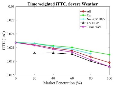
Figure 9 shows the performance of the iTTCtw of different vehicle types in severe weather scenarios. As shown in the severe weather scenario, when the CV MPR increases from 0 percent to 100 percent, the time-weighted iTTCtw of the passenger cars, HGVs, and all vehicles decrease by 12.24 percent, 23.82 percent, and 19.96 percent, respectively. When the CV MPR increases from 20 percent to 100 percent, the decrease of the iTTCtw is 14.92 percent for CVs and 11.04 percent for non-CVs. The safety improvement in terms of iTTCtw is the most significant in severe weather cases, less significant in snowy weather cases, and least significant in clear weather cases.
% = percent. CV = connected vehicle. HGV = heavy-goods vehicle. iTTC = inverse time-to-collision. s = second.
Source: FHWA
Figure 9. Chart. Time-weighted inverse time-to-collision under severe weather scenarios.
This graph has an x axis that is market penetration percent from 0 to 100, and a y axis for inverse time-to-collision as one over seconds squared from 0.015 to 0.03. Curves are drawn for all vehicles, cars, non-connected heavy-goods vehicles, connected heavy-goods vehicles, and total heavy-goods vehicles. The curves for all vehicles, cars, non-connected heavy-goods vehicles, and total heavy-goods vehicles all begin at 0 market penetration percent and about 0.022 inverse time to collision. The curve for connected heavy-goods vehicles begins at 20 market penetration percent and about 0. Points are plotted for all the curves at 0, 20, 40, 60, 80, and 100 percent market penetration, although the non-connected heavy-goods vehicles curve ends at 80 percent market penetration. The all curve ends at 0.018 and 100 percent. The car curve ends at 0.0195 at 100 percent. The total heavy-goods vehicles and controlled heavy-goods vehicles curves end at 0.017 at 100 percent. The non-connected heavy-goods vehicles curve ends 0.0195 at 80 percent.
Figure 10A and figure 10B show the average time distribution at each iTTC level during one trip in the network for the CV MPR of 0 percent and 100 percent. In all three weather scenarios, a vehicle spends most of the time under low-risk iTTC intervals (0.1 < iTTC < 0.2) and very little time under medium-risk (0.2 < iTTC < 0.3), high-risk (0.3 < iTTC < 0.4), and extreme-risk (iTTC > 0.4) intervals. The clear weather case involves more time at low-risk levels than that in snowy and severe weather cases, but involves the least time at the medium-to-extreme risk levels. In contrast, the severe weather scenario involves less time at the low-risk iTTC level, but much more time at the medium- and higher-risk levels than that in snowy and clear weather cases. In figure 10, when the charts are compared with the CV MPR of 0 percent and 100 percent, it is clear that, in addition to the overall safety risk reduction, the medium and higher risks with iTTC > 0.2 also significantly decrease. This indicates that implementation of TIMs can avoid many high-risk near-crashes, therefore considerably improving the overall system safety. Results also show the limited impact of mobility in terms of when the CV MPR increases. For all three weather scenarios, the increase in travel time when the CV MPR rises from 0 percent to 100 percent is only by 1.85 percent, 1.81 percent, and 1.12 percent, respectively. This indicates the effects of TIMs on mobility efficiency are limited.
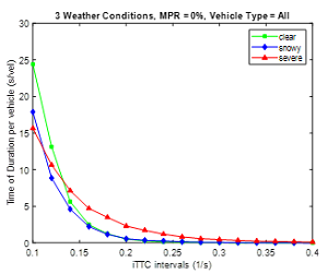
A. Chart. Connected vehicle market penetration rate = 0% scenario.
Graph has x axis of inverse time-to-collision per second from 0.1 to 0.4, and y axis of time of duration per vehicle in seconds per vehicle from 0 to 30. Three curves are plotted: clear, snowy, and severe for a connected vehicle market penetration rate of 0 percent. The curves at 0.1 inverse time-to-collision begin at: clear, 25 seconds per vehicle; snowy, 18 seconds per vehicle; and severe, 15.5 seconds per vehicle. All the curves slope steeply downward, then smoothly decrease to 0 vehicles per second at: 0.22 inverse time-to-collision per second for snowy and severe conditions, and 0.34 for clear conditions.
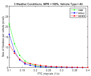
B. Chart. Connected vehicle market penetration rate = 100% scenario.
Graph shows x axis of inverse time-to-collision per second from 0.1 to 0.4, and y axis of time of duration per vehicle in seconds per vehicle from 0 to 30. Three curves are plotted on both graphs: clear, snowy, and severe for a connected vehicle market penetration rate of 100 percent. The curves at 0.1 inverse time-to-collision begin at: clear, 22 seconds per vehicle; snowy, 16 seconds per vehicle; and severe, 11 seconds per vehicle. All the curves slope steeply downward, then smoothly decrease to 0 vehicles per second at: 0.24 inverse time-to-collision per second for clear and snowy conditions, and 0.30 for severe conditions.
% = percent. iTTC = inverse time-to-collision. MPR = market penetration rate. s = second.
Source: FHWA.
Figure 10. Charts. Performance of inverse time-to-collision distribution from applying connected vehicles in different weather scenarios.
Variable Speed Limit
Figure 11 illustrates the results of the total iTTC for various scenarios when the CV MPR grows from 0 percent to 100 percent. The results show that for 0 percent TSR (i.e., non-CVs are not smoothed by CVs), the total iTTC increases when the CV MPR grows from 0 percent to 40 percent, indicating that system safety risks become higher. This is mainly because majority of the traffic on the roads is still non-CVs, and they will continue to drive fast before they see the VSL signs. Therefore, the interaction between fast non-CVs and slow CVs and maneuvers of lane changes and overtaking of non-CVs may result in many instances of high collision risks. Based on the results in this case study, the peak of the safety risks is reached at 40 percent of the CV MPR. After 40 percent, the iTTC curve of the 0 percent TSR starts to decline. This is because a sufficient number of CVs is on the road, and the CVs are able to block the overtaking maneuvers of upstream non-CVs. Therefore, the non-CVs are forced to follow CVs slowly, and the entire traffic is smoothed. Overall, when the CV MPR rises from 0 percent to 100 percent, the total iTTC of the 0 percent, TSR case decreases by 17.59 percent. When the TSR is 50 percent and 100 percent, the total iTTC drops with the increase of the CV MPR. The decreases in the total iTTC for 50 percent and 100 percent TSR cases when the CV MPR grows from 0 percent to 100 percent are 25.37 percent and 27.24 percent, respectively. The result indicates that CVs can induce the deceleration of non-CVs that follow the traffic-smoothing rule when the TSR is high. In high TSR cases, when a preceding CV slows down, the following non-CVs will drive more conservatively and tend to follow the new driving behavior of the front CVs. Such phenomena can then spread to the surrounding conservative non-CVs. Therefore, the overall trend of the total iTTC is downward with the growth of the CV MPR in the 50 percent and 100 percent TSR scenarios.
It is worth noting that when the CV MPR equals to 0 percent, the total iTTC under three TSR scenarios is different. As shown in figure 11, when the CV MPR is 0 percent, the total iTTC decreases with the growth of TSR. This is due to the difference in car-following modes between three TSR cases. Assume a vehicle slows down when observing a VSL sign (in all scenarios of this report, the assumed compliance rate with the VSL is 100 percent). If the following vehicles are conservative, they tend to follow the deceleration behavior of the preceding vehicle, even though the VSL sign is not yet within the sight distance. With more conservative vehicles in the network (i.e., higher TSR levels), the overall car-following behavior is smoother. Therefore, the collision risk of the traffic system can be mitigated with the rise of TSR even if CV MPR equals to 0 percent.
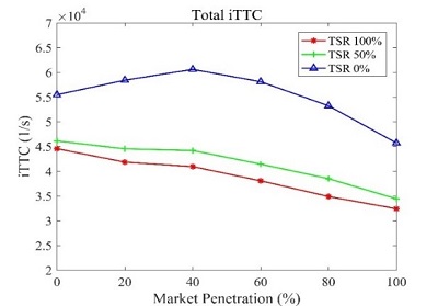
% = percent. iTTC = inverse time-to-collision. TSR = traffic smoothing rate. s = second.
Source: FHWA
Figure 11. Chart. Total inverse time-to-collision of all vehicles, cars, and heavy-goods vehicles under different traffic-smoothing rate percentages.
This graph has an x axis that is market penetration percent from 0 to 100, and a y axis for inverse time-to-collision per second from 2 times 10,000 to 7 times 10,000. Curves are drawn for traffic smoothing rates of 0, 50, and 100 percent. The curve for traffic smoothing rates of 0 starts at 5.5 at 0 percent, increases to 6 at 40 percent, and then declines to 4.5 at 100 percent. The curve for traffic smoothing rates of 50 starts at 4.6 and declines to 3.5 at 100 percent. The curve for traffic smoothing rates of 100 starts at 4.5 and declines to 3.25 at 100 percent.
Table 8 shows the decrease rate of the total iTTC of passenger cars and HGVs when the CV MPR rises from 0 percent to 100 percent under three TSR scenarios. Note that the total time-weighted iTTC shows similar trends. The decrease in the total iTTC for HGV is more significant than that of passenger cars because some HGVs are CVs, while all passenger cars are non-CVs. The decrease in the total iTTC of passenger cars indicates that when the TSR is at a high level, CV–VSL can also provide safety benefits to aggressive non-CVs whose behavior will not be smoothed unless they are blocked.
Table 8. The inverse time-to-collision reduction for cars and heavy-goods vehicles under three traffic-smoothing rate scenarios.
| Traffic-smoothing rate |
0% |
50% |
100% |
| Car |
8.00% |
17.02% |
18.28% |
| Heavy-goods vehicle |
21.96% |
29.27% |
31.50% |
Results also show that under three TSR scenarios, the increases in travel time as the CV MPR rises from 0 percent to 100 percent are limited. This indicates the limited impact of CV–VSL on system mobility efficiency.
In most scenarios in this case study, the increase of the CV MPR and TSR can both improve the safety performance of the traffic system, except when the CV MPR is at a low level and TSR is 0 percent. The changes in CV MPR and TSR cause no deterioration on the travel time performance, indicating that system mobility efficiency is not compromised.
Snowplow Pre-positioning
Table 9 shows the comparison of traffic performance between the base case and two pre-positioning cases. The weather condition is set to be severe in the simulation. To show the differences in performance under both low and high CV MPR, the results from two CV MPRs (20 percent and 80 percent) are compared in this case.
As shown in Table 9, both case 1 and case 2 pre-positioning outperform the base case in terms of iTTCtw and average travel time in either low or high CV MPR scenarios. Case 2 reduces the iTTCtw and average travel time more significantly than case 1. When the CV MPR is 20 percent, case 2 decreases 9.85 percent of iTTCtw of all types of vehicles, while case 1 only reduces 8.6 percent. When the CV MPR increases to 80 percent, the decrease in iTTCtw in case 2 rises to 10.38 percent, still larger than the 7.09 percent reduction in case 1. This is because case 2 distributes four snowplows far apart from each other and causes smaller impacts on other vehicles in the network.
Case 2 also leads to a decrease in average travel time as compared to the base case and case 1. The only measurement that case 1 outperforms case 2 is snowplow operation time. Case 1 reduces the operation time by 33.07 percent, while case 2 only decreases by 26.16 percent as compared to the base case. This is mainly because the snowplows in case 1 drive continuously along the freeway from start to end, while snowplows in case 2 change direction through interchanges during the plowing operation, and the times elapsed to traverse the interchange are included in the total operation time.
Table 9. Results of base case, case 1, and case 2 in severe weather.
| Case |
Base Case (20% CV) |
Case 1 (20% CV) |
Case 2 (20% CV) |
Base Case (80% CV) |
Case 1 (80% CV) |
Case 2 (80% CV) |
| iTTCtw of all types of vehicles (1/s²) |
0.02145 (0.00%) |
0.01960 (-8.60%) |
0.01934 (-9.85%) |
0.01018 (0.00%) |
0.00945 (-7.09%) |
0.00912 (-10.38%) |
| iTTCtw of passenger cars (1/s²) |
0.02181 (0.00%) |
0.02099 (-3.78%) |
0.02019 (-7.44%) |
0.01342 (0.00%) |
0.01266 (-5.65%) |
0.01232 (-8.22%) |
| iTTCtw of non-CV HGVs (1/s²) |
0.02200 (0.00%) |
0.01935 (-12.03%) |
0.01956 (-11.06%) |
0.01251 (0.00%) |
0.01213 (-3.01%) |
0.01195 (-4.45%) |
| iTTCtw of CV HGVs (1/s²) |
0.01849 (0.00%) |
0.01763 (-4.64%) |
0.01681 (-9.10%) |
0.00799 (0.00%) |
0.00734 (-8.10%) |
0.00705 (-11.77%) |
| iTTCtw of All HGVs (1/s²) |
0.02128 (0.00%) |
0.01900 (-10.69%) |
0.01896 (-10.89%) |
0.00878 (0.00%) |
0.00818 (-6.88%) |
0.00786 (-10.48%) |
| Average Travel Time (s) |
1,786.65 (0.00%) |
1,765.41 (-1.19%) |
1,760.26 (-1.48%) |
1,988.20 (0.00%) |
1,947.55 (-2.04%) |
1,954.58 (-1.69%) |
| Maximum Travel Time (s) |
2,076.34 (0.00%) |
2,102.83 (1.28%) |
1,957.57 (-5.72%) |
2,570.81 (0.00%) |
2,359.91 (-8.20%) |
2,322.84 (-9.65%) |
| Snowplow Operation Time (s) |
5,149 (0.00%) |
3,446 (-33.07%) |
3,802 (-26.16%) |
5,149 (0.00%) |
3,446 (-33.07%) |
3,802 (-26.16%) |
Summary
The simulation results show that effectiveness of all three CV WRMS strategies depends on weather conditions, CV MPRs, and the levels of impact of CVs on non-CVs (as quantified by using TSR in the study). Based on the simulation results, the following key observations and implications are summarized:
- AMS tools based on a microscopic traffic simulator have developed and proved effective in capturing realistic traffic and driving behavior under different weather conditions. It is also possible to implement and evaluate different WRMS that use RWIS and CV data as input, through a mapping between weather conditions, which is characterized by weather-related parameters (e.g., pavement condition, visibility, heavy snow) and various sets of driving behavior parameters (e.g., car-following gaps, look-ahead distance).
- For all scenarios, individual CV-based WRMS applications can improve traffic safety performance, as measured by iTTC. The effectiveness is most dramatic under severe weather conditions.
- TIMs can help improve the safety performance of the traffic system by reducing the risk of collisions and the occurrence of pileup crashes near the lane-closure event zones. In the I–80 case study, the CVs receive TIMs that include multiple advisories for the driver to decelerate or make lane changes to avoid potential collision with the preceding vehicles or objects in the lane-closure zones. The simulation results indicate that safety benefits provided by CVs continue to increase as the CV MPR rises.
- VSL can provide suitable speed limit advisories under different weather scenarios to keep vehicles driving at safe speeds. The weather information and road conditions can be obtained by RWIS stations, as well as vehicles equipped with weather sensors, to determine the safe speed limits correspondingly. The effectiveness of CV–VSL is influenced by both CV MPR and TSR. The safety performance improves as the rise of CV MPR at each TSR level. Meanwhile, the high TSR cases outperform the low TSR cases in safety performance, as measured by the iTTCtw of the traffic system under the same CV MPR.
- Snowplow pre-positioning is an effective strategy for winter surface maintenance that helps improve operation efficiency, reduce collision risks, and increase the mobility efficiency of the traffic system. Two pre-positioning strategies are designed and tested as compared to the base case. The multipoint positioning strategy is recommended for severe weather because it provides more performance benefits to the system, in terms of iTTC and travel time, than the other strategies. Either a two-point or multipoint pre-positioning strategy is acceptable for snowy weather because the performance difference is not significant for the two cases, indicating the average significant benefits if the pre-positioning of snowplows is implemented.
- For all three CV strategies, the level of safety benefits to the traffic system significantly depends on the weather scenarios. All three CV strategies tend to perform most effectively in severe weather. This is because when weather conditions are more severe (e.g., lower visibility, lower acceleration, and deceleration rate), there are more crash risks, and the advantages of CVs preventing large safety risks become more significant. With the TIMs updated continuously, the CV drivers can perform safer driving maneuvers under conditions in which non-CVs may be exposed to more substantial crash risks.
- The I–80 case study shows that when the CV MPR increases, though iTTC decreases in most cases, the travel time is not significantly impacted. In cases of snowplow pre-positioning in severe weather, the travel time performance even shows a non-negligible improvement with the growth of the CV MPR. This indicates that introduction of CVs to WRMS, which may even consist of strategies that slow down CVs, will at least maintain the same level of mobility efficiency of the system.
Suggestions for Additional Research
To further enhance the state of the practice and state of the art in using AMS tools for WRMS decision-making, the following future work, including research and deployment, are suggested:
- The AMS tool development in this project is designed as an framework to model CV technologies for traffic management, and three modules were developed and customized for specific WRMS. It is suggested to apply this framework to evaluate additional weather-responsive strategies in the future.
- The selected testbed in this case study has a traffic safety focus, and mobility-related performance is not as important. For congested traffic networks with adverse weather events, it would be necessary to fully implement the framework and develop customized simulation solutions, including additional modules such as online estimation and prediction of traffic demand. However, to ensure safety analysis at driver behavior level, microscopic simulations are still required.
- This case study uses a calibrated network from the Wyoming testbed. The simulation network is calibrated using weather and traffic detector data and can simulate three weather conditions: clear, snowy, and severe. It is recommended to use richer data sets, such as naturalistic driving data, to calibrate driver behavior models for a wider range of weather events. For example, WYDOT categorizes weather events into nine different types, and it is necessary to obtain nine sets of driving behavior parameters for each weather category to fully integrate such AMS models into the daily traffic management and maintenance operations.
- In this case study, the CV-based WRMS strategies are implemented and simulated in a virtual world in Vissim. All strategies are implemented in real time of the simulation. It would be of interest to directly test the simulation in selected TMCs. Two types of TMC integration are recommended. First, the offline AMS tool can be used by TMC staff to generate, in advance, an initial set of weather- and traffic-responsive strategies that will be applied when weather or traffic events occur, and continuously refined with real data. Second, for congested traffic networks where online simulation and decision-making are necessary, the AMS tool, or a customized one with less computational load for online implementation, can be applied to guide TMC operations in real time or near real time (i.e., tactical decision-making).
- The AMS tools usually require predictions of future traffic and weather conditions as inputs to simulate and evaluate the potential performance if certain strategies are implemented. It is suggested to integrate such systems with existing or new road condition prediction tools.