CHAPTER 5. METHODOLOGY AND FRAMEWORK
Note: Unless accompanied by a citation to statute or regulations, the practices, methodologies, and specifications discussed below are not required under Federal law or regulations.
Table 6 presents the five major components of the proposed calibration framework. These components will be presented throughout the main body of this chapter. For now, a high-level summary is provided. Although these components of the framework could indeed be applied individually or separately, applying the fuller set of components would likely achieve better models.
Table 6. Primary components of the calibration framework.
Calibration Concept |
Intent of Concept |
| Scenarios |
Calibrate unique models for typical combinations of demand, weather, and incidents. |
| Robustness |
Weighted sensitivity analysis of future demands and scenarios. |
| Parameter correlation |
Library of realistic driver types for different levels of aggressiveness. |
| Local density |
Develop relationships between driver behavior and degree of saturation. |
| Vehicle trajectories |
Comprehensive and compact representation of system performance. |
The first component is scenarios. Any robust calibration framework should address the highly variable nature of traffic demand, weather, incidents, work zones, and special events. Analysis of “typical” conditions is no longer considered safe, or helpful. In essence, there should be a unique simulation model created to represent, at the very least, each of the most common combinations of the above highly variable elements.
The second component is robustness. This component is important because analysis of future conditions is naturally governed by uncertainty. The level of uncertainty often relates to the lack of data. For example, the further into the future one wishes to forecast, the more uncertainty may exist around traffic demand levels. That said, future traffic demand levels may be more certain in some cities than others. Next, when it comes to analysis of emerging technologies (e.g., connected and automated vehicles) and traffic management strategies (e.g., advanced traffic demand management), the amount of available, relevant data may vary widely. For robust model parameters backed up by extensive data, a direct, highly confident calibration is possible. For uncertain model parameters having no data, the best that can be accomplished is a sensitivity analysis that accounts for all possibilities. For those model parameters backed up by, for lack of a better term, “medium” amounts of data, a Bayesian-style approach is needed. In this manner the model parameter is flagged with medium robustness, calibration accuracy is augmented by available data to the maximum possible extent, but a sensitivity analysis is nonetheless needed to forecast future possibilities.
The third component is parameter correlation. This component recognizes the pitfalls of calibrating model parameters independently, as if they were not correlated. If parameter correlations are not explicitly recognized or incorporated into the calibration process, fundamental soundness of the model may be compromised. For example, in a microscopic simulation model, the calibration process may produce driver type characteristics and profiles that do not exist in the real world. To mitigate this risk, a library of congruous model parameter settings should be provided. The prior chapter describes model parameters for microscopic, mesoscopic/macroscopic, and strategic models.
The fourth component is local density. This component recognizes the strong correlation between traffic congestion and driver behavior. The term ‘local density’ refers to the density of traffic in the local vicinity of a vehicle. Beyond this local spatial area, congestion levels would not affect driver behavior. However within the vicinity of a driver’s vehicle, the density of traffic in that area will profoundly affect their aggressiveness. Researchers believe a 500-foot radius around the vehicle is the best spatial area for predicting driver behavior. In cases where it is not possible to obtain densities near vehicle, a link-based or segment-based density may suffice, albeit with some loss of precision. The beauty of the local density concept is that the fundamental relationships between driver behaviors can be developed under existing conditions, and then re-used in future models having different densities on each segment.
The fifth and final component is vehicle trajectories. Use of trajectories in the calibration process is strongly encouraged for many reasons. Chief among these is that simulation models calibrated only to aggregate performance measures have been found to exhibit highly unrealistic driver behaviors.
OVERALL FRAMEWORK
Figure 18 in chapter 4 illustrates the proposed framework for the calibration process. As the first step, after refining the input data and performing an estimation process on the observed data, the appropriate set of parameters are selected/estimated. Simultaneously, the external conditions of the system are incorporated as exogenous input variables. In the proposed framework, the estimated parameters and external conditions are fed to the simulation model in terms of libraries of models, parameters, and related joint probabilities. These library components and probabilities would be used to develop various scenarios and agents as inputs for the simulation model. Using a set of scenarios and agents, the model will be calibrated based on the observations and forecast input variables collected from other sources such as census data.
An important difference between the conventional calibration process and the proposed calibration process is the manner in which the model is updated over time. The conventional approach involves a full re-calibration process when the model is applied to a new context. On the other hand, in the proposed framework, this computationally intensive process is avoided to some extent by updating the scenarios and libraries. Adaptive updating processes such as Bayesian techniques could be used to update the library parameters and their associated joint probability distributions.
LIBRARY OF PARAMETERS
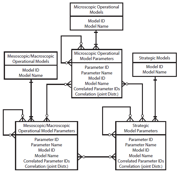
A key component of the framework is a library of parameters that act as a database accessed by the parameter estimator. Figure 45 shows the database structure for the library of parameters. The libraries could be classified into three major categories:
- Microscopic operational models and their associated parameters.
- Mesoscopic/Macroscopic operational models and their associated parameters.
- Strategic models and their associated parameters.
Each element in a parameter library is a parameter. Therefore, a unique key is assigned to each parameter. Besides the parameter ID, a model ID is also assigned to each parameter which represents the one-to-many relationship between the model library and the parameter library. This relationship is a mandatory relationship because every parameter belongs to a specific model defining the behavior of agents in the transportation system. Therefore, a parameter inherits the model attributes such as the conditions that are used to establish the validity of the model. On the other side of the one-to-many relationship, every model possesses at least one parameter that is stored in the respective parameter library.
One of the most important aspects of the proposed calibration methodology is preserving the correlation among the model parameters by defining joint probability distributions among the parameters. This is another attribute of a variable that should be stored in the parameter libraries. A set of correlated parameter IDs and their respective correlations represented as joint probability distribution functions could be stored in the parameter libraries. The recursive many-to-many relationships and the inter-library relationships symbolize the correlation among the model parameters. The recursive (intra-library) relationship captures the correlation among the parameters that belong to the same model category. For example, values of some parameters of a car following model could be associated with certain values of a lane changing model, when the models are utilized to simulate the behavior of an aggressive (or conservative) driver. The inter-library relationship captures the correlation among the parameters that belong to the different model categories. For instance, this correlation could exist among the parameters of the models used at different stages of the four-step model.
Source: FHWA, 2019.
Figure 45. Flowchart. Entity relationship diagram of the model parameter libraries.
The proposed data structure has the capability of introducing new models in the libraries. The model, as well as its parameters, should be added to the appropriate library categories. Once these parameters are entered in the database, they should be mapped to the other correlating parameters and the correlation should be defined using a joint distribution function. Besides adding a new element to the database, the attributes of each model and each parameter could be updated using adaptive processes as new data and observations become available over time. Bayesian techniques offer a formal framework for combining previous values with those based on new observations.
The structure also allows defining sets of deeper parameters that connect the initial parameter values to the scenarios attributes/features which is called reparameterization. The intent is for the deep parameters to remain valid over time. For example, the fraction of automated vehicles (market penetration) in the traffic mix could be made a parameter in the selection of an appropriate fundamental diagram for the corresponding scenario. Moreover, fundamental mechanisms and structural relations that are likely to remain valid as conditions change over time could be specified in the database. This rules out certain machine learning and data-driven approaches that involve training on specific datasets, and therefore have no ability to respond to structural change.
AGENT AND SCENARIO GENERATION PROCESS
Once the libraries of parameters are developed, samples could be drawn from the joint distributions
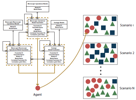
(or marginal distributions) of the parameters in order to generate agents with specified behavior. Based on the models selected for the sampling process, an agent could represent a vehicle, pedestrian, cyclist, or could represent a traffic control entity such as a traffic light, a ramp metering system, or a speed control system, or could be a representation of the condition in which the other agents interact in the specified transportation system; for example, the weather condition, the road network properties, or the road surface conditions, etc. A combination of agents generated in this manner would create a scenario that serves as an input of the simulation tool. This process is schematically shown in figure 46.
Source: FHWA, 2019.
Figure 46. Illustration. Process of generating agents and scenarios.
The left side of the figure contains the entity relationship diagram shown in figure 45. An agent is created by taking parameters from the following entities: microscopic operational model parameters, mesoscopic/macroscopic operational model parameters, and strategic model parameters. Three links are drawn starting from the three entities and ending at a circle representing an agent. On the right-hand side of the figure, several boxes are depicted. Each box represents a scenario and contains multiple items including circles, triangles, and rectangles. Each of these shapes symbolizes an agent in the system under the defined scenario.
Application of a transportation model for a future scenario would entail sampling/selecting from these libraries different agent types reflecting the particular mix expected. Generating different scenarios would essentially reflect the behaviors of these agents under various conditions. If there is certainty regarding the value of a parameter in the future, the parameter value would be the same through all generated scenarios. An example could be the geometric characteristics of the road network under consideration if, until the target year, there is not any major construction planned for the specified road segments.
SCENARIO-BASED ANALYSIS
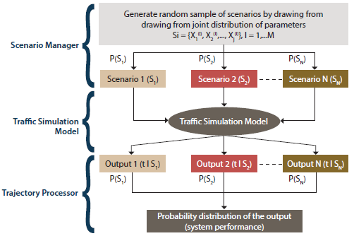
The method shown in figure 47 is useful when dealing with parameters that have some level of uncertainty.
Source: FHWA, 2019.
Figure 47. Flowchart. Scenario-based analysis.
In this situation, there is a limited set of values that is applicable to the parameters under consideration. The joint distributions (and correlations) among these parameters are known. The process combines different scenarios to generate the result of analyzing multiple scenarios. When there is enough information regarding the association between different sets of parameters deployed in the simulation tool, a joint distribution of parameter sets could be characterized. Random samples could be drawn from the set of scenarios using random sampling techniques such as the Monte Carlo methods. The sample size depends on the confidence level and anticipated errors in the respective scenarios. Each scenario, comprised of a different set of parameters, would be incorporated in the traffic simulation tool. The outputs of the simulation tool should be coupled with their respective scenario probability. In the trajectory processor step, these outputs should be combined with their associated weights (probabilities) to generate a probability distribution of the output under consideration. This approach is appropriate when there are some uncertainties involved but there is enough knowledge of the scenarios to generate a joint distribution of the scenarios. This approach could be useful to evaluate the transportation system under different demand distributions or under various incident scenarios.
ROBUSTNESS-BASED ANALYSIS
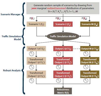
In contrast to the previous method, in some cases, there is a lack of information regarding the possible values of a parameter or the correlation among parameters. Examples of situations with such deep uncertainty could be fundamental changes to the transportation network environment at the target year, new transportation policies that have not been previously tested on the specific context, or introduction of new technologies such as connected and autonomous vehicles. As a result, a different approach should be used to combine the output of different scenarios when deep uncertainty exists. Instead of the joint distribution of the parameters, the marginal distributions might be known or assumed. As a result, the probability by which different scenarios occur is also unknown. As could be seen in figure 47 and figure 48, the main difference is in how the outputs of the simulation tool are treated. In the robustness-based analysis, according to a robustness measure selected by the analyst, the outputs are transformed and combined. The selection of the robustness metric depends on the suitability of the metric for the decision-context, the decision maker’s level of risk aversion, and the decision maker’s objective function, e.g., maximizing the performance measure or minimizing the variance of the performance measure. There are generally four types of robustness metrics: expected value metrics, metrics of higher orders (variance, skewness, and kurtosis), regret-based metrics, and satisficing metrics. Examples of these metrics and their pertinent transformations are provided in table 7 (McPhail, et al. 2018).
As shown in the graph, three levels of transformation are performed to transform the performance measure output of the simulation tool to a specified robustness metric. First, a system performance transformation (T1) is conducted to derive a value that is more compatible with the robustness metric (for example, change the travel time to regret-based congestion as the difference between the travel time of the selected scenario and the free flow travel time). Then, a scenario subset selection (T2) is performed that selects a subset (one/a few/all) of the scenarios based on the robustness metric and desired level of risk aversion (for example, the 75th, 80th, 90th percentiles among travel time of all scenarios). The robustness metric calculation is the third transformation. This step combines the values derived in the previous steps for the selected scenarios to calculate the robustness metric for the scenarios (for example, the expected value/skewness/kurtosis of the calculated robustness metric for the selected scenarios). A list of sample robustness metrics that would be used in this study is shown in table 6. The “identity” cells mean that no specific transformation is performed at the stage and the performance value is directly passed to the next step.
Source: FHWA, 2019.
Figure 48. Flowchart. Robustness-based analysis.
Table 7. Transformations for robustness metrics.
| Robustness Metric |
T1 |
T2 |
T3 |
| Maximin |
Identity |
Worst case |
Identity |
| Maximax |
Identity |
Best case |
Identity |
| Laplace’s principle of insufficient reason |
Identity |
All |
Mean |
| Hurwicz optimism-pessimism rule |
Identity |
Worst and best cases |
Weighted mean |
| Minimax regret |
Regret |
Worst case |
Identity |
| Nth percentile minimax regret |
Regret |
Nth percentile |
Identity |
| Undesirable deviations |
Regret |
Worst-half cases |
Summation |
| Percentile-based skewness |
Identity |
10th, 50th, and 90th percentiles |
Skew |
| Percentile-based peakedness |
Identity |
10th, 25th, 75th, and 90th percentiles |
Kurtosis |
Source: McPhail et al. 2018.
CONCLUSIONS
This chapter has presented the framework proposed for calibrating traffic operational models and simulation tools for application to future conditions. The framework is predicated on four key notions: (1) That the models themselves are responsive to the features of the future scenario (i.e., that the descriptors that specify a particular scenario be included in the model specification); (2) the definition of a library of model parameters corresponding to different types of agents under varying conditions; (3) the role of scenarios in both specifying future conditions of interest as well as triggering certain ranges of parameter values for those scenarios; and (4) the potential for robustness analysis in situations where uncertainty about future scenarios or conditions is large.