CHAPTER 4. CALIBRATION NEEDS
Given the assessments of calibration methodologies and data presented in the previous chapters, this chapter presents a gap analysis. The analysis will identify a set of traffic analysis tool calibration needs for transportation improvement evaluations, and describe the impacts of these gaps. The set of calibration needs is intended to provide a “snapshot” of the potential updates that may be beneficial for the current calibration methods.
Note: Unless accompanied by a citation to statute or regulations, the practices, methodologies, and specifications discussed below are not required under Federal law or regulations.
GAP ANALYSIS AND GAP IMPACTS
Current calibration practices mostly use statistical, econometric, or optimization techniques to find parameter values that make model outputs best match the available data. Calibration, inherently, requires knowledge and observation/measurement of actual conditions. When comparing the model outputs to the data representing the actual conditions of the system, it is typically assumed that the relations established at the calibration stage would remain valid in the future under new system conditions. Therefore, the model specifications and parameters are assumed to remain unchanged. The only changes considered for future conditions are in the values of the variables that serve as input for the simulation model. The values of variables are typically forecast independently or determined as the result of an intervention. These assumptions limit the effectiveness of the simulation tool in capturing the system behavior under the future conditions and desired interventions.
Whenever there are uncertainties or heterogeneity associated with model parameters considered in the calibration process, the typical process is to draw samples from the set of parameter values using the marginal probability distributions of the parameters. As the sampled parameters are inserted into the simulation tool, unrealistic behavior could appear in the system output. One of the reasons for the unrealistic behavior is the correlation existing among the parameters which could not be captured when the samples are taken from the marginal probability distributions.
IMPACTS OF THE GAPS
The limiting assumption regarding the consistency of the parameter values in the calibration stage and those under the future conditions of the system has two major effects. First, the calibrated model is unable to capture the system performance under future conditions and policy interventions. The other impact is that a more reliable understanding of the transportation system could be achieved only if a full re-calibration process is performed. Therefore, the computationally expensive calibration should be repeated more frequently as the previously calibrated model become ineffective when applied to a new area and context.
The main influence of ignoring the correlations among parameters incorporated in the simulation model is that unrealistic behavior could evolve in the simulated environment; hence the reliability of the model would be decreased.
Based on the impact of the gaps in the current calibration practices, the main challenge is how to ensure that the model specifications and parameter values used in applying the model to predict traffic system performance under the future scenario of interest are adequate; i.e., that the model is “calibrated for future conditions.” Of course, since these future conditions have not yet occurred at the time the model is used, it is not possible to directly observe actual conditions for such scenarios as a basis for model calibration. Addressing this challenge involves a significant shift in the mindset of traffic modelers: from model estimation and calibration aimed at replicating existing and past conditions to greater emphasis on prediction quality and accuracy. A new calibration framework should be developed that intrinsically encompasses this mindset shift. The necessary elements of the proposed framework are discussed in the following section.
CALIBRATION NEEDS
The main problem addressed in this study is how to develop and calibrate models so that the output they produce is meaningful and provides a realistic and accurate depiction of future conditions. In order to address this problem, there are several elements that should be incorporated in the calibration tools.
First, libraries of models and parameters associated with each model should be added to the calibration framework. These libraries contain different values for the parameters as well as an estimated probability distribution for the set of values. The library items are constructed based on historical data and forecast values for future conditions not been realized yet. Table 3 provides an example of three well-known car-following models with their parameters. The traffic analysis tool should have the capability of updating the library of models and parameters as new possible sets of values for parameters and new behavioral models are introduced.
Table 3. Parameters of three car-following models.
Model |
Parameter |
Description |
| Gipps |
T |
Reaction time. |
a |
Maximum acceleration. |
d |
Maximum desirable deceleration (<0). |
V* |
Desired speed. |
s* |
Minimum net stopped distance from the leader. |
α |
Sensitivity factor. |
| Helly |
T |
Reaction time. |
C1 |
Constant for the relative speed. |
C2 |
Constant for the spacing. |
d* |
Desired net stopped distance from the leader. |
γ |
Constant for the speed in the desired following distance. |
| IDM |
a |
Maximum acceleration. |
b |
Desired deceleration. |
V0 |
Desired speed. |
s0 |
Minimum net stopped distance from the leader. |
THW |
Desired safety time headway. |
IDM = intelligent driver model.
Second, the correlations among elements of the libraries should be integrated into the calibration tool. The correlations could be represented as joint probability distributions for vectors of parameters. Throughout the calibration process, selecting the model parameters from the joint probabilities instead of the marginal probabilities of each individual parameter could reflect more realistic behavior of the simulation agents.
As shown in figure 17, combining the libraries of parameters related to different components of the transportation system (demand-related, expected supply-related, and unexpected supply-related components) and selecting from the library values based on the joint probabilities of the selected parameters defines a single scenario/agent block. A scenario is defined by set of operational conditions (reflecting external events, such as weather, demand surges, etc.), interventions (infrastructure changes, control actions, dynamic system management schemes, etc.), as well as characteristics of the general activity system (land use, activity locations) and associated technologies (e.g. connected and autonomous vehicles, Internet of Things, smart cities). On the other hand, an agent is an object in the simulation environment that follow a set of rules defined by various behavioral models. The behavioral characteristics of an agent are defined by the parameters of the agent’s behavioral models.
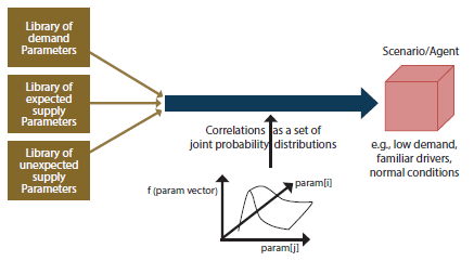
Source: FHWA, 2019.
Figure 17. Illustration. Process of developing a scenario/agent.
The third useful element for the calibration of traffic analysis tools is trajectory-based data. As mentioned earlier, one of the main aspects of the new calibration procedure is a significant shift from model estimation and calibration based on existing and past conditions, to greater emphasis on prediction quality and accuracy. To perform this fundamental change, a higher quality and more accurate input data set should also be used. The trajectories of agents (vehicles, pedestrians, bicyclists, etc.) could provide such a level of accuracy through continuous monitoring of the agent behavior over time and space. The simulation tools should become capable to receive trajectories of agents as an input data. As small errors in processing trajectory-based data could result in significant errors in the model outputs, appropriate preprocessing techniques and error handling methods should be included in the algorithms of the simulation tool.The third useful element for the calibration of traffic analysis tools is trajectory-based data. As mentioned earlier, one of the main aspects of the new calibration procedure is a significant shift from model estimation and calibration based on existing and past conditions, to greater emphasis on prediction quality and accuracy. To perform this fundamental change, a higher quality and more accurate input data set should also be used. The trajectories of agents (vehicles, pedestrians, bicyclists, etc.) could provide such a level of accuracy through continuous monitoring of the agent behavior over time and space. The simulation tools should become capable to receive trajectories of agents as an input data. As small errors in processing trajectory-based data could result in significant errors in the model outputs, appropriate preprocessing techniques and error handling methods should be included in the algorithms of the simulation tool.
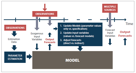
Figure 18 shows the proposed framework for the calibration process. As the first step, after refining the input data and performing an estimation process on the observed data, the appropriate set of parameters are selected/estimated. Simultaneously, the external conditions of the system are incorporated as exogenous input variables. In the proposed framework, the estimated parameters and external conditions are fed to the simulation model in terms of libraries of models, parameters, and related joint probabilities. These library components and probabilities would be used to develop various scenarios and agents as inputs for the simulation model. Using a set of scenarios and agents, the model will be calibrated based on the observations and forecast input variables collected from other sources such as census data.
Source: FHWA, 2019.
Figure 18. Flowchart. Proposed calibration framework.
In general, the longer the horizon over which a scenario is defined, i.e., the further out into the future one is trying to forecast, the greater the uncertainty associated with the values of input variables. This is especially true not only for the activity system variables and the associated technologies but also the social fabric and associated preferences/lifestyles/norms. Furthermore, as the horizon becomes longer, there is a need for a more diversified set of scenarios and agents in the calibration process.
A major difference between the conventional calibration process and the proposed calibration process is the manner that the model is updated over time. The conventional approach involves a full re-calibration process when the model is applied to a new context. On the other hand, in the proposed framework, this computationally intensive process is avoided to some extent by updating the scenarios and libraries. Adaptive updating processes such as Bayesian techniques could be used to update the library parameters and their associated joint probability distributions.
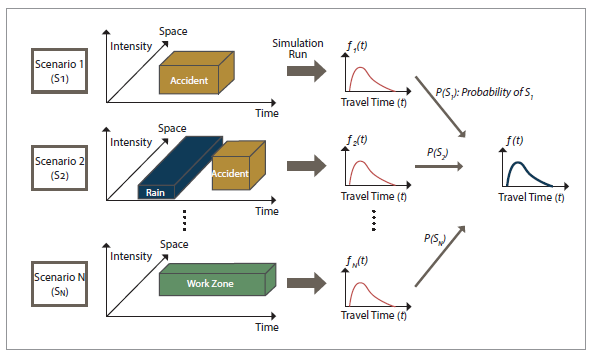
As illustrated in figure 19, probability distributions of the model outputs are developed based on the
probability distributions assigned to the scenarios. The outputs of the scenarios are combined using
the probability assigned to each scenario in order to generate the final probability distribution of the
output. If a comprehensive list of scenarios and agents are considered in the calibration process, as
new observations are collected over time, the probabilities assigned to the agents and scenarios
could be revised. Consequently, the probability distributions of the outputs could be adjusted
accordingly. Throughout this updating process, there would be no need to perform a full recalibration
process and the updates would be directly applied to the inputs and outputs. In the
proposed framework, a re-calibration process could become necessary if the conditions of the new
observations are not covered in the set of scenarios/agents or if a new behavioral model is
introduced to the transportation system.
© Kim, Mahmassani, Vovsha, et al., 2013.
Figure 19. Illustration. Constructing model output (travel time) distribution based on
scenario-specific simulation outputs.
CALIBRATION NEEDS LIBRARIES
The first element introduced in the above framework is the libraries of models and parameters. Libraries could be classified into libraries of microscopic, mesoscopic, macroscopic, strategic models. The libraries listed in this section constitutes well-known models which are thoroughly studied in the literature. The final traffic analysis calibration tool should be able to accommodate new models introduced as new technologies are introduced (new modes, new fuels or propulsion technologies, connected and/or automated vehicles), or major changes are implemented in the operation of the transportation system. As the macroscopic and mesoscopic relations reflect the underlying microscopic behaviors of the drivers in a particular setting, it is important to consider the correlations that exist between the macroscopic, mesoscopic, and microscopic parameters. Therefore, besides the correlations that exist among the parameters of a specific library, there are correlations across libraries that are defined for various analysis levels (micro, meso, and macro).
CALIBRATION NEEDS FOR OPERATIONAL MODELS: MICROSCOPIC
Microscopic models of driver behavior in traffic capture the maneuvers of individual drivers as they interact in traffic, including car following, acceleration choice, lane changing, merge decisions, gap acceptance, and queue discharge headways. The model parameters in this case typically capture psychological aspects of driver behavior, including risk attitudes. When using a calibrated model for prediction under new contemplated scenarios, the main factors assumed to change are the situational variables describing respective vehicle positions and speeds. However, parameters governing these behaviors are known to change across drivers and vehicle characteristics (heterogeneity), which in turn vary across locations and over time. Similarly, these are affected by operational conditions such as rain, snow, and visibility.
To deal with this variability, libraries of parameter values may be developed reflecting behaviors under different conditions. Furthermore, it is expected that new vehicle technologies, especially connected and/or automated vehicles will have a major impact on microscopic behaviors. Therefore, libraries related to the microscopic behavior of vehicles should be enhanced as new models and new parameter values are introduced. Car-following models are among the most important models characterizing the microscopic behavior of vehicles. The Newell model is one of simplest car- following models in which the follower imitates the leader trajectory with a lag in time and space. Therefore, it is also known as a trajectory translation model (Punzo and Simonelli 2005).
Figure 20. Formula. Newell car-following model (trajectory translation model).
The location of the follower vehicle (n) at a specified time plus the reaction time (x subscript n (open parenthesis) t plus T (close parenthesis)) equals the position of the leader vehicle (n minus 1) at the specified time (x subscript n minus 1 (open parenthesis) t (close parenthesis)) minus the follower desired intervehicle spacing (d subscript n).
The Gipps model is a safety distance model that considers the safe speed in two different regimes: the free-flow regime and the car-following regime (Kim and Mahmassani 2011).
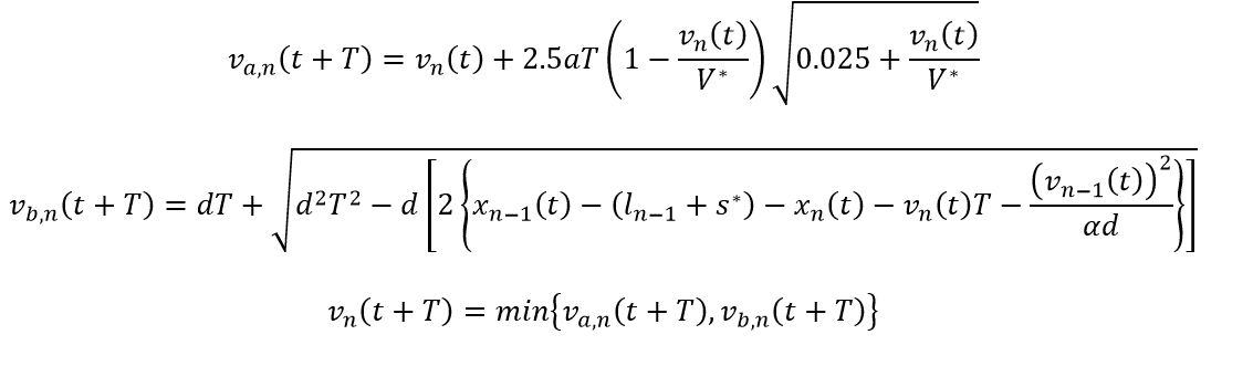
Figure 21. Formula. Gipps car-following model.
The Helly model is a linear model that relates the acceleration of the follower to the speed difference and spacing between the leader and follower considering the reaction time as the time step (Kim and Mahmassani 2011).
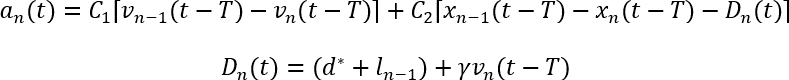
Figure 22. Formula. Helly car-following model.
The intelligent driver model (IDM) is a continuous response model which considers the follower’s acceleration to be a continuous function of the leader’s speed, and spacing and speed differences between the two vehicles. A major difference between this model and the other models introduced in this section is that the IDM does not consider any reaction time in the formulation (Kim and Mahmassani 2011).
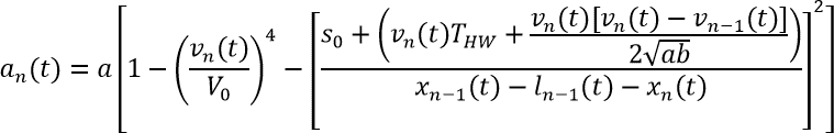
Figure 23. Formula. The Intelligent Driver Model.
Last but not least, a stimulus-response acceleration model implemented in the MITSIMLab (MIT Intelligent Transportation Systems sIMulation Laboratory) microsimulator. It combines sensitivity and the effect of a stimulus to produce the relevant response (Punzo and Simonelli 2005).
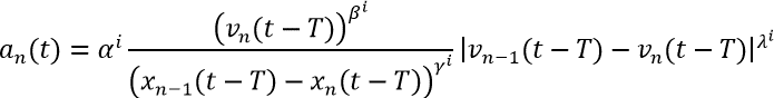
Figure 24. Formula. The stimulus-response acceleration model in MITSIMLab.
Where xn (t+T) and xn-1(t) represent the follower and leader positions, respectively; vn(t+T) and vn-1(t) represent the follower and leader speeds, respectively. Similarly, an(t+T) and an-1(t) are the follower and leader accelerations, respectively. T is the reaction time; dn is the desired intervehicle spacing; a is the maximum acceleration; d is the maximum desirable deceleration; V* represents the desired speed; ln is the physical length of vehicle; s* is the minimum net stopped distance from the leader; α is the sensitivity factor; d* is the desired net stopped distance from the leader; C1, C2,and γ are constant parameters related to the relative speed, spacing, and speed in the desired following distance, respectively; b is the desired deceleration; Vo is the desired speed; so is the minimum net stopped distance from the leader; THW symbolizes the desired safety time headway; and ai, βi, γi, and λi are eight parameters related to the car-following regime (with i specifying whether the follower is in acceleration or deceleration mode).
Another important set of microscopic models in the traffic flow is the lane-changing and merging decision models. Rahman et al. (2013) classified the lane-changing models into four groups: rule- based models, artificial intelligence models, incentive-based models, and discrete-choice-based models. The Gipps model, the model implemented in CORSIM (CORridor SIMulation), the ARTEMiS (Analysis of Road Traffic and Evaluation by Micro-Simulation) model, the cellular automata model, and the game theory-based models are examples of the rule-based models.
Examples of artificial intelligence models are the models developed based on the fuzzy logic or based on an artificial neural network structure. MOBIL (Minimizing Overall Braking Induced by Lane changes) , as an incentive-based model, is a lane-changing model that combines the attractiveness of a given lane defined by a utility function and the risk associated with the lane- changing maneuver, which is compared to a safety criterion. There are various parameters in the definition of the utility function describing the attractiveness. Furthermore, other parameters could be involved in the combination of the incentive and risk measures. LMRS (Lane-Changing Model with Relaxation and Synchronization) is another example in the incentive-based model category. This model performs a trade-off between the route, speed, and keep-right incentives. The following equation shows one way of combining these incentives to measure the driver’s desire to change lane:
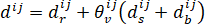
Figure 25. Formula. The Lane-Changing Model with Relaxation and Synchronization.
The combined desire to change lane from i to j (d superscript ij) equals the desire to follow a route (d superscript ij subscript r) plus a voluntary (discretionary) incentive (theta superscript ij subscript v) multiplied by the result of adding the desire to gain speed (d superscript ij subscript s) to the desire to keep right (d superscript ij subscript b).
Where dij is the combined desire to change lanes from i to j;  is the desire to follow a route;
  is the desire to gain speed;
  is the desire to keep right; and
  is voluntary (discretionary) incentive which is a parameter that needs to be determined and adjusted based on the available context.
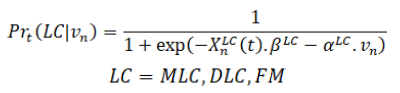
Figure 26. Formula. A probabilistic model for lane changing.
Where Prt(LC|vn) is the probability of executing MLC, DLC, or FM for driver n at time t;  is a vector of explanatory variables affecting decision to lane changes; βLC is the corresponding vector of parameters; vn is the driver-specific random term; and αLC is the parameter associated with the random term. Jia et al. (2011) estimated and validated the parameters of involved in this formulation using traffic data collected from a typical urban expressway merging section in Guangzhou. They used the lead gap, the lag gap, the relative speed of the lead vehicle to the subject vehicle, the relative speed of the subject vehicle to the lag vehicle, the subject speed, the remaining distance, and driver characteristics as the explanatory variables in the merging probability model.
Gap acceptance models, similar to the lane-changing behavior, possess a rule-based or a probabilistic framework. Mahmassani and Sheffi (1981) proposed a gap acceptance model using a standard cumulative normal distribution mathematical formula as follow:
Figure 27. Formula. A gap acceptance model based on standard cumulative normal distribution.
In this equation, the probability of accepting gap i in the sequence of gaps (Pr (open parenthesis) accept gap i vertical bar T bar subscript cr, beta, delta, i, t subscript i (close parenthesis)) equals the cumulative probability of a standard normal distribution when the Z-value is equal to (open parenthesis) the gap duration (t subscript i) minus the average critical gap when facing the first gap (T bar subscript cr) minus a model parameter beta multiplied by the result of i minus 1 to the power of another model parameter delta (close parenthesis) divided by the variance across drivers and gaps (sigma).
Where Φ(.) denotes the standard cumulative normal curve; i is the sequential number of the gap; ti is the gap duration;  is the average critical gap when facing the first gap; β and δ are parameters that need to be estimated and subsequently calibrated based on the context that the model is being utilized; and σ is the variance across drivers and gaps.
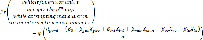
Taylor and Mahmassani (1998) proposed a gap acceptance model with a structure similar to the above formulation. They used the model to characterize the gap acceptance behavior of bicyclists and motorists with a probit mathematical formulation but with different estimated parameters.
Source: FHWA.
Figure 28. Formula. A probit gap acceptance model for bicyclists and motorists.
Where Φ(.) denotes the standard cumulative normal curve; dgvmi represents the actual gap duration; βo is the mean critical gap when all other attributes are zero; Xgap is a vector of attributes characterizing the gap and surrounding events; Xint is a vector of attributes characterizing the intersection environment; Xman is a vector of attributes characterizing the acting vehicle maneuver; is a vector Xvo of attributes characterizing the vehicle/operator unit; Xia is a vector of interactions between attributes from different groups; βgap, βint, βman, βvo, and βia is the total variance across vehicle/operator units, gaps, maneuvers, and intersection types.
Finally, the queue discharge models, that explain the queue discharge behavior under stochastic capacity scenarios at freeway bottlenecks, play a significant role in determining the performance of freeway systems. Jia et al. (2010) proposed a robust and easily implementable methodology that identifies freeway bottlenecks and models the queue discharge behavior at the bottlenecks. They formulated the queue discharge rate as a stochastic time-correlated recursive formula. It was implemented in DYNASMART-P using the following functional form:
Figure 29. Formula. Queue discharge rate in DYNASMART-P.
In this equation, the queue discharge rate at time interval t (C subscript t) equals the queue discharge rate at time interval t minus 1 (C subscript t minus 1) plus a model parameter (beta) times (open parenthesis) the average discharge rate (mu subscript c) minus the queue discharge rate at time interval t minus 1 (C subscript t minus 1) (close parenthesis) plus a normally distributed random term (epsilon subscript t).
Where Ct is the queue discharge rate at time interval t; β is parameter that should be estimated and calibrated; μc is the average discharge rate; and εt is a normally distributed random term that is added to consider the stochasticity nature of the problem.
Table 4 summarizes the microscopic model parameters introduced in this section that should be calibrated. There are various other models that could be added to the listed microscopic models.
Table 4. Parameters of microscopic models.
Model |
Parameter |
Description |
CAR-FOLLOWING MODELS |
| Newell |
T |
Reaction time. |
dn |
Desired intervehicle spacing. |
| Gipps |
T |
Reaction time. |
a |
Maximum acceleration. |
d |
Maximum desirable deceleration (<0). |
V* |
Desired speed. |
s* |
Minimum net stopped distance from the leader. |
α |
Sensitivity factor. |
| Helly |
T |
Reaction time. |
C1 |
Constant for the relative speed. |
C2 |
Constant for the spacing. |
d* |
Desired net stopped distance from the leader. |
γ |
Constant for the speed in the desired following distance. |
| IDM |
a |
Maximum acceleration. |
b |
Desired deceleration. |
V0 |
Desired speed. |
s0 |
Minimum net stopped distance from the leader. |
THW |
Desired safety time headway. |
| MITSIM |
αi |
Parameter for the car-following regime (i represents acceleration/deceleration). |
βi |
Parameter for the car-following regime (i represents acceleration/deceleration). |
γi |
Parameter for the car-following regime (i represents acceleration/deceleration). |
λi |
Parameter for the car-following regime (i represents acceleration/deceleration). |
LANE-CHANGING MODELS |
LMRS
Ahmed (1999) |
|
Voluntary (discretionary) incentive. |
βLC |
Vector of parameters in the lane-changing model. |
αLC |
Parameter associated with the random term. |
| Jia et al. (2011) |
Dlead |
Lead gap. |
Dlag |
Lag gap. |
ΔVlead |
Relative speed of the lead vehicle to the subject vehicle. |
ΔVlag |
Relative speed of the subject vehicle to the lag vehicle. |
Vsub |
Subject speed. |
Dram |
Remaining distance. |
δsub |
Driver characteristics. |
GAP ACCEPTANCE MODELS |
| Mahmassani and Sheffi (1981) |
Tcr |
Average critical gap when facing the first gap. |
β |
Parameter in the gap acceptance model. |
Δ |
Parameter in the gap acceptance model. |
| Taylor and Mahmassani (1998) |
β0 |
Mean critical gap when all other attributes are zero. |
βgap |
Parameter related to the gap and surrounding events. |
βint |
Parameter related to the intersection environment. |
βman |
Parameter related to the acting vehicle maneuver. |
βvo |
Parameter related to the vehicle/operator unit. |
βia |
Parameter related to the interactions between attributes from different groups. |
QUEUE ACCEPTANCE MODELS |
| Jia et al. (2010) |
β |
Parameter in the queue discharge model. |
IDM = intelligent driver model. LMRS = Lane-Changing Model with Relaxation and Synchronization.
MITSIM - MIcroscopic Traffic SIMulator.
CALIBRATION NEEDS FOR OPERATIONAL MODELS: MESOSCOPIC AND MACROSCOPIC
Fundamental diagrams capture the relation between flow, density, and speed. They are widely used to represent flow propagation in mesoscopic simulation-based dynamic network assignment tools. A calibrated fundamental diagram can characterize the performance of the respective facility and/ or network in a robust manner.
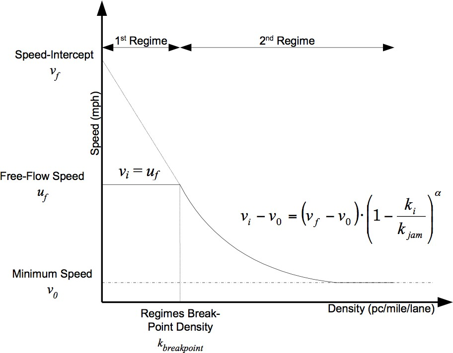
The Greenshields models in DYNASMART are the traffic flow models that needs to be calibrated based on the desired context (Mahmassani, Hou, et al. 2014). The Type 1 model is a dual-regime model with a constant free-flow speed for the free-flow conditions and modified Greenshields model for congested-flow conditions as shown in figure 30. The Type 1 model is applicable to freeways because it can accommodate dense traffic (up to 23,000 passenger cars per hour per lane (pc/hr/ln)) at near free-flow speeds.
Source: FHWA, 2019.
Figure 30. Graph. Type 1 modified Greenshields model (dual-regime model).
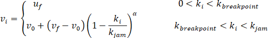
The following equation mathematically specifies the Type 1 modified Greenshields model:
Figure 31. Formula. Type 1 modified Greenshields model.
Where vi is the speed on link i; vf is the speed-intercept; uf is the free-flow speed on link i; vo is the minimum speed on link i; ki is the density on link i; kjam is the jam density on link i; kbreakpoint is the breakpoint density; and a is the power term.
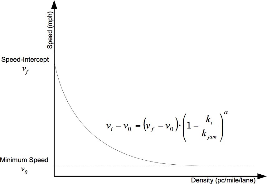
The Type 2 model is a single-regime Greenshields model that models both the free- and congested- flow conditions using a single relation as shown in figure 32. This model is more appropriate for arterials.
Source: FHWA, 2019.
Figure 32. Graph. Type 2 modified Greenshields model (single-regime model).
The graph plots density (x-axis) against speed (y-axis). Passenger car per mile per lane (pc forward slash mile forward slash lane) is selected as the unit for density and miles per hour (mph) as the unit for speed. A convex decreasing curve is depicted that possesses an intersection point called the speed-intercept (v subscript). The speed on the curve asymptotically diminishes to the minimum speed (v subscript 0). The formula in figure 33 is shown in the graph.
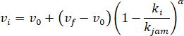
The Type 2 modified Greenshields model is expressed in the following mathematical equation:
Figure 33. Formula. Type 2 modified Greenshields model.
The speed on link i (v subscript i) equals the minimum speed on link i (v subscript 0) plus (open parenthesis) the speed intercept (v subscript f) minus the minimum speed on link i (v subscript 0) (close parenthesis) times (open parenthesis) 1 minus the density on link i (k subscript i) divided by the jam density (k subscript jam) (close parenthesis) to the power of a model parameter alpha.
In the above modified Greenshields models, the combination of values and joint probability distributions of vf, uf, vo, kjam, kbreakpoint, and a constitutes a library of parameters for the modified Greenshields models that should be calibrated.
There are other fundamental diagram relationships whose parameters could be added to the libraries of parameters in the proposed framework. For example:
- Greenberg’s logarithmic model defined as
Figure 34. Formula. Greenberg’s logarithmic model.
- Underwood’s exponential model defined as
Figure 35. Formula. Underwood’s exponential model.
Where ko is the optimal density which is a parameter that needs to be calibrated.
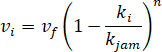
- Pipes’ generalized model defined as
Figure 36. Formula. Pipes’ generalized model.
The speed on link i (v subscript i) equals the speed intercept (v subscript f) times (open parenthesis) 1 minus the density on link i (k subscript i) divided by the jam density (k subscript jam) (close parenthesis) to the power of a model parameter n.
Where n is a parameter that needs to be calibrated.
One of the features of DYNASMART is the capability to consider the effect of weather condition on the following supply-side parameters (Mahmassani, Hou, et al. 2014):
- Traffic flow model parameters: speed-intercept, minimal speed, density breakpoint, jam density, and the shape term alpha;
- Link performance: maximum service flow rate, saturation flow rate, and posted speed limit adjustment margin;
Left-turn capacity: g/c ratio;
- 2-way stop sign capacity: saturation flow rate for left-turn vehicles, saturation flow rate for through vehicles, saturation flow rate for right-turn vehicles;
- 4-way stop sign capacity: saturation flow rate for left-turn vehicles, saturation flow rate for through vehicles, saturation flow rate for right-turn vehicles; and
- Yield sign capacity: saturation flow rate for left-turn vehicles, saturation flow rate for through vehicles, saturation flow rate for right-turn vehicles.
The weather-sensitive Traffic Estimation and Prediction System (TrEPS) is implemented in DYNASMART to accurately estimate and predict the traffic status under various weather conditions. The effect of weather condition is captured using a corresponding weather adjustment factor (WAF) as
Figure 37. Formula. Weather effect adjustment of model parameters in DYNASMART.
Where fiweather event is the value of parameter i under a certain weather condition, finormal represents the value of parameter i under normal weather condition, and Fi is the WAF for parameter i.
The WAF could be defined as a linear function of weather conditions combining the effect of visibility and precipitation intensity as the following mathematical formula:
Figure 38. Formula. Weather adjustment factor as a function of weather condition.
Where v is visibility; r is precipitation intensity of rain; s is precipitation intensity of snow; and βio, βi1, β;i2, βi3, βi4, βi5, are the coefficients within the WAF function that need to be estimated and calibrated based on the context and the study area characteristics. Comprehensive libraries of these coefficients could be implemented in traffic analysis calibration tools. More coefficients could be added to the libraries as more complex correlations between the WAF of a traffic supply-related parameter and the weather-related variables are identified.
CALIBRATION NEEDS FOR STRATEGIC MODELS
Strategic models possess a higher level of complexity compared to operational models. Choice dimensions such as route choice, mode choice, and departure time choice are the main contributors in the complexity of strategic models. There is an extensive body of literature, in the transportation area, on choice models and strategies that could influence the behavior of individuals. The main emphasis of this section is on choice models that considered the effect of different transportation management strategies. Examples of strategic models from the literature are provided in the remainder of this section.
Frei et al. (2014) integrated demand models into weather-responsive network traffic estimation and prediction system methodologies. Therefore, the system encompasses weather-responsive traffic management (WRTM) strategies as well as active travel demand management strategies such as pre-trip information dissemination and rescheduling of school hours. Since the WRTM strategies aim short- to medium-term decisions, the behavioral choice dimensions that could be influenced by travel demand management strategies are route choice, departure time choice, and mode choice.
Their proposed framework has three parts:
- A base travel demand model with travel time and cost skims calibrated using multicriteria dynamic user equilibrium.
- A network-level scenario manager with weather adjustment factors to update the travel time and cost skims according to the adjusted supply values using multicriteria dynamic user equilibrium.
- A disaggregated demand model that gets updated based on the updated disaggregated user time and cost skims.
Eventually, the framework output influences the short- and medium-term traveler decisions. One of the models they developed using this framework was a departure time choice model that contains a scheduling cost function (Cs) defined as follows:
Figure 39. Formula. Scheduling cost in a demand model proposed by Frei et al. (2014).
The scheduling cost (C subscript s) equals the alternative specific constant for departure time plus a cost parameter (beta subscript 1) times (open parenthesis) the free flow travel time (T) plus the extra travel time caused by recurrent congestion (T subscript w) (close parenthesis) plus a cost parameter (beta subscript 2) times the schedule delay early (SDE) plus a cost parameter (beta subscript 3) times the schedule delay late (SDL).
Where T is the travel time defined as the summation of free-flow travel time and extra travel time caused by recurrent congestion; SDE is the schedule delay early; SDL is the schedule delay late; β1, β2, and β3 are cost parameters to be estimated and calibrated, referring to the cost of travel time per unit of time, cost per unit of time for arriving early, and cost per unit of time for arriving late, respectively; and const denotes the alternative specific constant for departure time that should be estimated and calibrated.
Highway tolling and pricing strategies are among the strategies that are extensively studied to capture their effect on travelers’ behavior. In the traditional four-step trip-based models, pricing has a first-order impact on the trip mode and trip time of day choice dimensions. It has a second-order impact on trip generation and trip distribution models. On the other hand, for the activity-based models, it has a first-order impact on the trip mode, tour mode, and tour time of day choice dimensions. The second-order impact of pricing for the activity-based models appears in the tour primary destination and tour generation models (Perez, Batac and Vovsha 2012).
Perez et al. (2012) proposed a generalized cost function to evaluate the utility of each network link of a route according to the following formula:
Figure 40. Formula. Link-level cost function proposed by Perez et al. (2012).
The generalized cost for the vehicle type and auto occupancy class k (G subscript k) equals a model coefficient for travel time (beta subscript 1k) times the travel time for the vehicle type and auto occupancy class k (T subscript k) plus a model coefficient for travel cost (beta subscript 2k) times the travel cost including toll for the vehicle type and auto occupancy class k (T subscript k).
Where k refers to the vehicle type and auto occupancy class; Tk is the travel time; Ck is the travel cost including the toll; and β1k and β2k are coefficients for travel time and travel cost that should be estimated and calibrated.
A more generalized version of the above cost function could be formulated in order to incorporate other choice dimensions such as the mode choice utility function.
Figure 41. Formula. A generalized mode choice utility function.
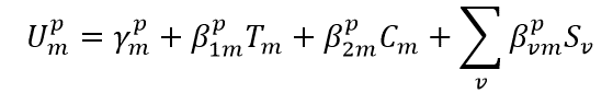
Where m represents the set of modes including auto occupancy classes; p is the travel purpose and other possible segments; v refers to the person, household, and zonal variables; Tm is the travel time by mode; Cm is the travel cost by mode; Sv symbolizes the person, household, and zonal variables;  is the mode-specific constant for each trip purpose/segment; and the parameters that need estimation and calibration are
  which are the coefficients for travel time, travel cost, and person/household/zonal variables by travel mode and trip purpose/segment.
The Logsum of the utility function for the mode choice model could be used to generate the impedance functions of upper-level choice dimensions such as the time-of-day choice and destination choice models. The time-of-day choice utility function could be formulated by adding the Logsums of the utility function for the mode choice model in the following manner:
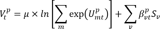
Figure 42. Formula. A time-of-day choice utility function.
The time-of-day choice utility for trip purpose p at time of day period t (V superscript p subscript t) equals a model parameter (mu) time the natural logarithm of the summation over all travel modes of the exponential of the mode choice utility for the trip purpose p traveled by the mode m at time of day period t (U superscript p subscript mt) plus the summation over all individuals/households/zones for the following multiplication: a model coefficient for the person/household/zonal effect by time of day period and trip purpose/segment (beta superscript p subscript vt) times the person/household/zonal variable (S subscript v).
Where  is the mode choice utility for the trip purpose p traveled by the mode m at time of day period t, and μ and
  are the parameters that need to be estimated and calibrated. The parameter μ is a scaling factor that possesses a value in the unit interval.
Similar to the time-of-day choice model, the destination choice utility function could be written as:
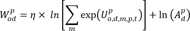
Figure 43. Formula. A destination choice utility function.
The destination choice utility for trip purpose p from zone o to zone d (W superscript p subscript od) equals a model parameter (eta) time the natural logarithm of the summation over all travel modes of the exponential of the mode choice utility for the trip purpose p traveled from zone o to zone d using the mode m at time of day period t (U superscript p subscript o,d,m,p,t) plus the natural logarithm of the destination zone attraction for the trip purpose p (A superscript p subscript d).
Where

refers to the mode choice utility for the trip purpose
p traveled from zone
o to zone
d using the mode
m at time of day period
t;

is the destination zone attraction (size variable) for each trip purpose, such as total employment for work purpose, enrollment for school purposes, and retail employment for non-work purpose; and
η is a parameter, possessing a value in the unit interval, that needs to be estimated and calibrated.
Reliability is another important aspect that should be incorporated in choice dimension models. It represents the uncertainty level with respect to congestion levels and travel time. More reliable alternatives are generally preferred because of various reasons including but not limited to negative consequences of late arrival at the destination, needing a buffer time to avoid late arrival, and discomfort caused by the uncertainty of travel time at a given time. Therefore, incorporating reliability variables in choice dimension models could potentially improve the model performance.
Vovsha et al. (2013) proposed a generalized model as the highway utility function that includes basic components such as time and distance as well as a reliability-related component. The cost of path is incorporated in a non-linear way to account for the effects of income and vehicle occupancy. They formulated the highway utility function as follows:
Figure 44. Formula. Highway utility function proposed by Vovsha et al. (2013).
The highway utility equals an alternative-specific constant for tolled facilities (delta) plus a model parameter (beta subscript 1) multiplied by the average travel time (Time) times (open parenthesis) 1 plus a model parameter (beta subscript 2) times the travel distance (D) plus a model parameter (beta subscript 3) times the square of the travel distance (D) (close parenthesis) plus a model parameter (beta subscript 4) times the monetary cost of using the facility including the tolls, parking, and fuel (Cost) over the multiplication of the household income of the traveler to the power of a model parameter (beta subscript 5) and the vehicle occupancy to the power of a model parameter (beta subscript 6) plus a model parameter (beta subscript 7) times the day-to-day standard deviation of the travel time (STD) over the travel distance (D).
Where Δ is the alternative-specific constant for tolled facilities; Time is the average travel time; D is the travel distance; Cost refers to the monetary cost of using the facility including the tolls, parking, and fuel; I is the household income of the traveler; O indicates the vehicle occupancy; STD is the day-to-day standard deviation of the travel time. There are seven parameters (β1, β2, . . ., β7) that should be estimated and calibrated to fully specify the model.
The authors listed 11 key behavioral insights, which are useful for implementing transportation management strategies, that could be derived from the values estimated and calibrated for the parameters (Vovsha, et al. 2013):
- Variation in the value of time (VOT) across highway users.
- Income and willingness to pay.
- Vehicle occupancy and willingness to pay.
- Constraints on time-of-day shifting.
- Importance of value of reliability (VOR) and its association with VOT.
- Effect of travel distance on VOT and VOR.
- Evidence of negative toll bias.
- Hierarchy of likely responses to change in tolls and congestions.
- Summary of user segmentation factors.
- Avoiding simplistic approaches to forecasting.
- Data limitations and Global Positioning System-based data collection methods.
Table 5 summarizes the strategic model parameters introduced in this section that should be calibrated. There are various other models that could be added to the listed strategic models.
Table 5. Parameters of strategic models.
Model |
Parameter |
Description |
SCHEDULING COST FUNCTION |
| Frei et al. (2014) |
β1 |
Cost of travel time per unit of time. |
| β2 |
Cost per unit of time for arriving early. |
| β3 |
Cost per unit of time for arriving late. |
SIMPLE ROUTE UTILITY FUNCTION |
| Perez et al. (2012) |
β1k |
Coefficient for travel time of vehicle type k. |
| β2k |
Coefficient for travel cost of vehicle type k. |
MODE CHOICE UTILITY FUNCTION |
| Perez et al. (2012) |
|
Mode-specific constant for each travel mode and purpose/segment. |
 |
Coefficient for travel time for each travel mode and purpose. |
 |
Coefficient for travel cost for each travel mode and purpose. |
 |
Coefficient for person, household, and zonal variables for each travel mode and purpose. |
TIME-OF-DAY CHOICE UTILITY FUNCTION |
| Perez et al. (2012) |
μ |
Scaling coefficient that should be in the unit interval. |
|
Coefficient for person, household, and zonal variables for each travel purpose and time of day. |
DESTINATION CHOICE UTILITY FUNCTION |
| Perez et al. (2012) |
η |
Scaling coefficient that should be in the unit interval. |
HIGHWAY UTILITY FUNCTION |
| Vovsha et al. (2013) |
β1 |
Coefficient for travel time. |
| β2 |
Coefficient reflecting the impact of travel distance on the perception of travel time. |
| β3 |
Coefficient reflecting the impact of travel distance on the perception of travel time. |
| β4 |
Coefficient for travel cost. |
| β5 |
Coefficient reflecting the impact of income on the perception of cost. |
| β6 |
Coefficient reflecting the impact of occupancy on the perception of cost. |
| β7 |
Coefficient reflecting the impact of travel time reliability. |
The strategic models introduced here are a few examples of various models available in the literature. Compared to the operational models discussed in previous sections, development of libraries for these models is more challenging. Various strategies not only impact the value of the variables used in the formulation but also could influence the parameter values. As a result, extensive libraries of strategic models should be produced by combining different management strategies, external conditions (e.g., weather conditions and incidents), and internal behavioral characteristics of simulation agents. These libraries could be used to generate the desired scenarios. In this case, a scenario would be essentially a set of strategies, models, and parameters.
CONCLUSIONS
There are several issues in the conventional calibration processes that reduce the effectiveness of the simulation model, prevent the applicability of the models to new areas and context, and produce unrealistic behavior. These issues could be addressed by introducing new elements in the calibration framework such as libraries of models, parameters, and relevant joint probability distributions capturing correlation effects among the parameters. Besides these elements, using trajectory-based data could improve the quality and accuracy of the model outputs. Last but not least, the adaptive updating process is another feature in the proposed framework that could reduce the computational effort for the calibration process.
Three categories of models were introduced: microscopic operation models, mesoscopic and macroscopic operational models, and strategic models. Developing comprehensive libraries of models and parameters is an essential component of the proposed calibration framework. As a result, a data structure should be constructed to maintain these libraries. The capability of updating the models and parameters of these libraries and the correlation among these libraries would be clearly specified in the proposed data structure.