CHAPTER 3. DATA ASSESSMENT
A fundamental element of traffic analysis tool (TAT) application is the supporting data that enables tool calibration, validation, and validity of results for evaluating the transportation improvements. Calibrating Traffic Analysis Tools to conditions that are ultimately evaluated involves data from improvements that may not be deployed yet. This challenge is magnified for evaluating emerging technologies and strategies that have not been mainstreamed into our transportation networks (e.g., advanced transportation demand management, integrated corridor management, and connected and automated vehicles). Since these emerging technologies and strategies are not yet widespread, this chapter aims to assess the practical issues and impacts relating to data, both existing and future.
This chapter identifies and documents what data sources exist, or are likely to be available in the future, for the transportation improvement being evaluated. This will also include data sources that may be promising, or that may require transformation, in meeting objectives where no suitable data is anticipated to be available in the near term.
Note: Unless accompanied by a citation to statute or regulations, the practices, methodologies, and specifications discussed below are not required under Federal law or regulations.
DATA COLLECTION TECHNIQUES
The objective of calibration a traffic simulation model is to estimate the parameter values that establish the structural relations, amongst the relevant variables, that govern the behavior of the system. Validation further verifies the ability of the model to replicate and predict traffic conditions given specific inputs such as the traffic demand, operational control strategies and interventions, and external environmental factors. Errors in the collected data could influence the simulation in two different ways. First, errors in the raw data influence the outputs derived from the simulation tool. Second, estimated error-prone variables compared to simulation results could impact the optimal set of parameter values estimated as a result of the calibration process.
Therefore, the model input should be carefully checked and pre-processed prior to the calibration of model parameters.
Daamen et al. (2014) classified the data used in traffic simulation studies into six groups:
- Local detector data.
- Section data (vehicle re-identification).
- Vehicle-based trajectory data.
- Video-based trajectory data.
- Behavior and driving simulation.
- Stated and revealed preferences.
The first two data groups primarily reveal macroscopic properties of the system. The last two typically address individual behavior, at the microscopic level; driving simulation data could synthetically reflect driver’s behavior at a microscopic level. On the other hand, the trajectory data (vehicle-based and video-based) could be used for both microscopic and macroscopic studies.
However, the main limitations associated with the trajectory data are the limited coverage in terms of the number of vehicles equipped with tracking devices (for the vehicle-based trajectory data) and the limited spatial coverage (for the video-based trajectory data). Emerging technologies in the vehicle connectivity area both in the vehicle-to-vehicle and vehicle-to-infrastructure communication could address these limitations. Since the trajectory data is more informative than the other types of data, the calibration of simulation models that deal with car-following, lane changing behaviors, and other microscopic behaviors should be more emphasized.
DATA PROCESSING AND ENHANCEMENT
The data collected to serve as an input for the simulation tool should be filtered, aggregated, and corrected before the calibration and validation processes. As a first step, data should be processed, and data fusion techniques should be used (when dealing with multiple data sources) to generate an estimate of the traffic state of the system. Typical techniques in this stage are digital filters, least square estimation, expectation maximization methods, Kalman filters, and particle filters. In the second step, features and patterns that would be used to compare the results of the simulation model for calibration purposes should be derived from the preprocessed data. Classification and inference methods are the common techniques utilized in this step. Examples of these techniques are statistical pattern recognition, Dempster-Shafer, Bayesian methods, neural networks, correlation measures, and fuzzy set theory. Last but not least, the key input of the simulation tool should be specified (Daamen, Buisson and Hoogendoorn 2014).
Two types of error are usually seen in raw trajectory data: random error and systematic error. The noise in trajectory data is magnified when the position information is converted to speed and acceleration through a differentiation process. This is an example of random errors that can happen in trajectory data. On the other hand, the cumulative distance traveled by a vehicle is usually overestimated. The bias is a non-negative, non-decreasing function of the number of observations. The magnitude of this error increases as the speed of the vehicle decreases. This is an example of a systematic error in the trajectories. The space error in trajectory also becomes important when the interaction of vehicles is considered such as in car-following or lane changing models. Platoon consistency is the term defined in this area that verifies the consistency of the following vehicles and the traveled space. This error could be resolved by projecting coordinates on the road lane alignment (Punzo, Borzacchiello, and Ciuffo 2011).
As mentioned earlier, the calibration of the collected data is an import step toward reaching reliable results from the simulation tool. The way of performing this calibration also influences the accuracy of the resulting preprocessed data. For example, the vehicle trajectory positions (1) could be smoothed first then differentiated to get velocities and accelerations; (2) could be differentiated first and then all three types of data could be smoothed simultaneously; (3) a sequential process could be undertaken that smooths the positions then derives velocities, then smooths velocities and derives the accelerations afterwards. The preservation of internal consistency should be considered in any of these calibration processes. To be more specific, the integration of speed and acceleration should return the measured travel space (Daamen, Buisson and Hoogendoorn 2014).
One of the main limitations in assessing the accuracy of calibrating trajectory techniques (averaging, smoothing, Kalman filtering, Kalman smoothing) is that there is no established method that can quantify the level of accuracy. This is an important issue even with a large dataset such as the NGSIM data (Daamen, Buisson and Hoogendoorn 2014).
Macroscopic traffic data sensors such as loop detectors, radar, or infrared sensors, and cameras are prone to both random errors (noise) and structural errors (bias). Since data assimilation techniques are ineffective in resolving structural errors, other techniques such as speed bias correction algorithms should be used to address this issue (Daamen, Buisson and Hoogendoorn 2014).
For instance, one of the most common errors is to use time mean speed instead of space mean speed when deriving other traffic state parameters. The relationship between these two parameters could be written as:
Figure 6. Formula. Relationship between time mean speed and space mean speed.
Where vt is the time mean speed, vs is the space mean speed, and σs is the variance of space speed. The variance is an unknown quantity in this formula, and the contribution of the second term could reach up to 25 percent in congested conditions. As a result, directly using the time mean speed to derive other traffic flow characteristics, such as density and flow, results in systematic biases (Daamen, Buisson and Hoogendoorn 2014).
ROLE OF VEHICLE TRAJECTORIES IN THE TAT CALIBRATION PROCEDURE
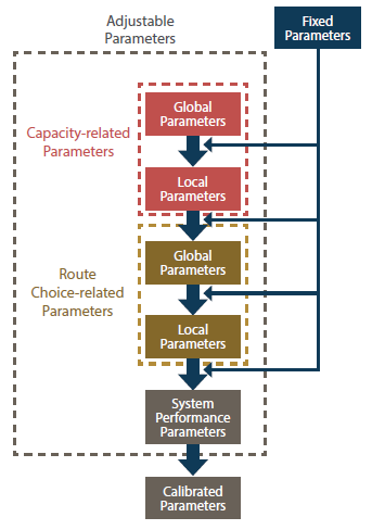
The traffic analysis toolbox (Dowling, Skabardonis, and Alexiadis 2004) suggests a step-by-step calibration procedure. Figure 7 shows the procedure schematically. As could be seen in the figure, the parameters that serve as inputs for the simulation tool are divided into two groups of adjustable and fixed parameters based on a trade-off between the computational effort required for the calibration and the degree of freedom for fitting the calibrated model to the local conditions. The adjustable parameters are further subdivided into parameters that influence the system capacity and parameters that influence the route choice. These two groups of parameters could be further subdivided into global parameters and local parameters. As a sequential process, first, the global capacity-related parameters are calibrated by analyzing the queue discharging points at the network bottlenecks. Average following headway, driver reaction time, critical lane changing gap, minimum separation in the stop-and-go situation, startup lost time, queue discharge headway, and gap acceptance for unprotected left turns are examples of parameters that directly affect the capacity.
Then, the model is fine-tuned by adjusting local parameters such as the presence of on-street parking, driveways, or narrow shoulders. The next step involves adjusting the global and local parameters that directly influence the route choice until the link volumes are best fitted to the collected data. Examples of global route choice-related parameters are route weightings for travel time and travel cost, drivers’ familiarity with different each route, and the error in the drivers’ perception of the cost and time for each route. The last step in the calibration process is to modify some link free-flow speeds and link capacities. The modification should be limited in order to avoid significant deviations of the model behavior from the behavior derived from the capacity-related and route choice-related calibration steps. The aim of the system performance calibration is to achieve certain goals when model performance estimates are compared to field measurements.
Examples of these calibration targets are the statistical thresholds for traffic flows, travel times, and the visual audits for link speeds and bottlenecks which are used by Wisconsin Department of Transportation (DOT) for its Milwaukee freeway system simulation model.
Source: FHWA, 2019.
Figure 7. Flowchart. The traffic analysis tools calibration procedure.
Sufficient information about vehicle trajectories could be very helpful in this sequential calibration process. The vehicle trajectories could not only specify the bottlenecks of the system but also could evaluate the capacity of the system at the queue discharging points. Both vehicle-based and video- based trajectory data provide useful information for the capacity-related model calibration stage. For the route choice-related parameters, the behavior of the drivers could be studied through the data collected by a vehicle-based trajectory data collection system.
LOCAL DENSITY THROUGH VEHICLE TRAJECTORIES
The vehicle trajectories could be processed to derive a variety of system performance metrics. An important system performance measure which is used in many traffic information systems is the traffic density. The commonly used vehicle density estimation that is designed based on infrastructure-based traffic information systems suffers from low reliability, limited spatial coverage, high deployment cost, and high maintenance cost. Another approach for estimating the road density is to use information derived from vehicle trajectories. This approach becomes more reliable as more vehicle become equipped with sensors and wireless technologies, and the connectivity level increases in vehicular ad-hoc networks (VANET).
The following formula shows the relationship between density and space mean speed in Pipes proposed a car-following model.
Figure 8. Formula. Relationship between density and space mean speed.
Where λis the vehicle interaction sensitivity, and kjam is the jam density.
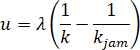
In the two-fluid theory, space mean speed could be calculated by the following formula:
Figure 9. Formula. Space mean speed in the two-fluid theory.
Space mean speed (u) equals the allowed maximum speed (u subscript max) multiplied by (open parenthesis) 1 minus the fraction of stopped vehicles (f subscript s) (close parenthesis) to the power of 1 plus the indicator for service quality of vehicular networks (nu)."
Where umax is the allowed maximum speed, fs is the fraction of stopped vehicles, and ν is an indicator for service quality of vehicular networks.
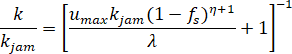
Combining the above equations would result in a mathematical relationship between road density and the fraction of stopped vehicles as follows:
Figure 10. Formula. Relationship between road density and fraction of stopped vehicles.
Density (k) over jam density (k subscript jam) equals the inverse of (open bracket) 1 plus the allowed maximum speed (u subscript max) times the jam density (k subscript jam) divided by the vehicle interaction sensitivity parameter (lambda) multiplied by (open parenthesis) 1 minus the fraction of stopped vehicles (f subscript s) (close parenthesis) to the power of 1 plus the indicator for service quality of vehicular networks (nu) (close bracket).
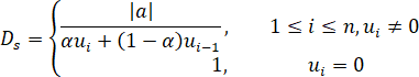
Artimy (2007) used the ratio of stopping time to trip time for probe vehicles as an estimator for the fraction of stopped vehicles. In another study, Luo et al. (2017) proposed a velocity and acceleration aware density estimation algorithm to estimate the neighboring density of a vehicle with known trajectory using the vehicle acceleration and velocity:
Figure 11. Formula. Density as a function of velocity and acceleration.
The neighboring density of a vehicle (D subscript s) equals the absolute value of the acceleration/deceleration divided by the result of the summation of alpha times the speed at time step i (u subscript i) plus 1 minus alpha times the speed at time step i minus 1 (u subscript i minus 1), when the speed at time step i (u subscript i) is not equal to zero. The time step varies from one to the total number of time steps (n). The parameter alpha is equal to one when the vehicle is accelerating and zero when the vehicle is decelerating. When the speed at time step i (u subscript i) is equal to zero, the neighboring density of a vehicle (D subscript s) equals 1.
Where i represents a time step, and a is equal to one when the vehicle is accelerating and zero when it is decelerating.
In order to convert the real-time local density to the road segment density, averaging techniques could be utilized, or the segment length should be short enough to avoid significant variations in the estimated local density values. One of the main limitations stated by both studies is the inaccuracy of the local density estimate in free-flow traffic conditions.
Simpler techniques also exist to estimate the density of a road segment using the local density around vehicles that can collect information of their surrounding area. One approach is to use the inverse of the average inter-vehicular spacing. The other approach is to find the density of the vehicles in the area that could be visualized by the vehicle sensors. The analysis would be performed on a case study to infer the road segment density from local density values.
DATA REQUIREMENTS
One of the main data requirements, which serves both on the input side as a basis for calibration of the simulation model parameters, and on the output side to perform validation, is the vehicle trajectory data. Mahmassani et al. (2014) enumerate trajectory information requirements as follow:
- Provide at least longitude and latitude (or X-Y) coordinates with associated timestamps.
- Capture a wide range of operational statuses such as recurring and nonrecurring congestion.
- Cover a wide range of road facilities from freeways to arterial roads and intersections.
- Include sufficient sampling and time-series to support statistically meaningful analysis.
- Provide the capability of fusing other ancillary data with the trajectory data.
Satisfactory knowledge over the trajectories, the independent behavior of simulation agents, and the interactions between agents in the simulation environment could support the development of libraries of agents with attributes associated with them representing the agent behavior in the simulation environment. The heterogeneity among members of an agent class could be defined via a probabilistic distribution as an attribute for the agent class or the agent could be further divided into subagent classes.
Beside the endogenous effects that could be derived from the underlying interaction between vehicle trajectories, another important source of information used in the simulation is related to exogenous sources of variability, such as policy interventions, traffic incidents, construction zones, special events, and weather conditions. These datasets are usually provided by transportation authorities that are in charge of the management, control, or monitoring of transportation systems or by third parties such as meteorological organizations. Table 2 shows the data used to characterize exogenous sources of variability. Libraries of scenarios corresponding to different operational conditions could be created based on relevant historical data.
Table 2. Typical data elements for exogenous sources of variation in system performance measures.
Event Type |
Data Elements |
| Incident |
- Type (e.g., collision, disabled vehicle).
- Location.
- Date, time of occurrence, and time of clearance.
- Number of lanes/shoulder and length of roadway affected.
- Severity in case of collision (e.g., damage only, injuries, fatalities).
- Weather conditions.
- Traffic data in the area of impact before and during the incident (e.g., traffic flows; speed, delay, travel time measurements; queues; and other performance measures or observations, if available).
|
| Work zone |
- Work zone activity (e.g., maintenance, construction) that caused lane/road closure, and any other indication of work zone intensity.
- Location and area/length of roadway impact (e.g., milepost), number of lanes closed.
- Date, time, and duration.
- Lane closure changes and/or other restrictions during the work zone activity.
- Weather conditions.
- Special traffic control/management measures, including locations of advanced warning, speed reductions.
- Traffic data upstream and through the area of impact, before and during the work zone (e.g., traffic flows and percentage of heavy vehicles; speed, delay, travel time measurements; queues; and other performance measures or observations, if available).
- Incidents in work zone area of impact.
|
| Special event |
- Type (e.g., major sporting event, official visit/event, parade) and name or description.
- Location and area of impact (if known/available).
- Date, time, and duration.
- Event attendance and demand generation/attraction characteristics (e.g., estimates of out-of-town crowds, special additional demand).
- Approach route(s) and travel mode(s) if known.
- Road network closures or restrictions (e.g., lane or complete road closures, special vehicle restrictions) and other travel mode changes (e.g., increased bus transit service).
- Special traffic control/management measures (e.g., revised signal timing plans).
- Traffic data in the area of impact before, during, and after the event (e.g., traffic flows; speed, delay, travel time measurements; queues; and other performance measures or observations, if available).
|
| Weather |
- Weather station identification or name (e.g., KLGA1 for the automated surface observing system station at LaGuardia Airport, New York).
- Station description (if available).
- Latitude and longitude of the station.
- Date, time of weather record (desirable data collection interval: 5 minutes).
- Visibility (miles).
- Precipitation type (e.g., rain, snow).
- Precipitation intensity (inches per hour, liquid equivalent rate for snow).
- Other weather parameters (temperature, humidity, precipitation amount during previous 1 hour, if available).
|
Source: Mahmassani, Kim, et al., 2014.
1 KLGA is the four-letter International Civil Aviation Organization designation for at LaGuardia International Airport and its associated weather station.
DATA STRUCTURE
As mentioned in the review and assessment of calibration methodologies, the correlation between input parameters is an important factor that should be considered. The correlation among the parameters could be captured through a joint probabilistic distribution assigned to the parameters. In general, the type of parameters that would be used in this project could be classified into three groups as follows:
- Type 1: Parameters with the least level of uncertainty.
- Type 2: Parameters with some level of uncertainty.
- Type 3: Parameters with deep uncertainty.
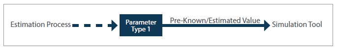
The first type of parameters pertains to most of the parameters available in the base year that capture the behavior of different agents in the normal prevailing condition of the system in the absence of new technologies. The heterogeneity among the individuals in the same agent class is preserved through an assigned probabilistic distribution or a sub-classification of the agent. The least uncertainty level exists in the parameter values and the interaction effects. Historical data and predefined libraries of agents could be used to determine or estimate the values of these parameters (figure 12). The data still should be preprocessed to remove random errors and systematic biases.
Source: FHWA, 2019.
Figure 12. Illustration. Parameters with the least level of uncertainty [type 1].
The flowchart possesses three labeled entities linked by unidirectional arrows. The first entity ('estimation process') is connected to the second entity (rectangle named “parameter type 1”) representing that throughout the estimation process the parameters type 1 are generated. Then, the “parameter type 1” box is connected to the third entity ('simulation tool'). This connection shows that pre-known or estimated values for the type 1 parameters are entered the simulation tool.
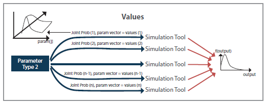
The second type of parameters imposes more uncertainty on the analysis. The uncertainty could be related to the value of the parameters such as the unknown composition of risk-averse and risk- taking individuals among the drivers when the cognitive aspects are incorporated in the car- following models (Hamdar, et al. 2008). The uncertainty could also be attributed to the correlation between parameters. For example, there are uncertainties involved when the effect of exogenous sources that cause variations in the system performance measures. Examples are mentioned in table
1. In this case, a library of scenarios is available and through sampling techniques, such a Monte Carlo sampling, the values, and associated probabilistic distributions would be selected. The sampled sets would be entered in the simulation tool and the outputs would be processed and combined to develop probabilistic distributions of system performance measures (figure 13).
Source: FHWA, 2019.
Figure 13. Illustration. Parameters with some level of uncertainty [type 2].
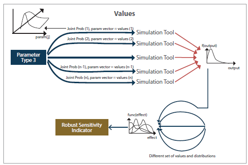
The third type of parameters encompasses the highest level of uncertainty. This case is relevant to emerging technologies in the transportation system such as autonomous vehicles and innovative control strategies in connected environments. In this case, the parameter values, the correlation effects, and the joint probabilistic distributions are unknown. A process similar to the scenario- based value development for parameters type 2 should be performed for parameters type 3.
However, due to the high level of uncertainty in the values and joint distributions, a robust sensitivity approach is utilized. Several criteria from decision theory have been used in the literature to perform robust sensitivity analysis when a large number of scenarios should be analyzed, namely, the maximax, the weighted average, the minimax regret, and the limited degree of confidence (Gao and Bryan 2016, Gao, Bryan and Nolan, et al. 2016).
The maximax decision criterion (Smax) first finds the maximum possible payoff (gain or loss) for each scenario. For example, the maximum travel time for a specific path or the least capacity for a specific link. Then, it selects the scenario that has the highest maximum payoff as the selected scenario. The weighted average decision criterion (Savg) is utilized when multiple performance measures are considered simultaneously, and the sensitivity indicators are combined with appropriate weights to calculate an overall sensitivity indicator that could be used to specify the selected scenarios. The minimax regret decision criterion (Sreg) is a commonly used criterion in decision theory. Regret is defined as follows:

Figure 14. Formula. Regret formulation.
Minimum value among all the scenarios defined based on type 3 parameters of the maximum regret occurred among all the scenarios defined for type 1 and type 2 parameters (minimum function over scenarios with type 3 parameters (a) of maximum function over scenarios with type 1 and type 2 parameters (b) for r subscript a,b) is equal to the minimum among all the scenarios defined based on type 3 parameters of the maximum among all the scenarios defined for type 1 and type 2 parameters of the absolute difference between the system performance measure under the presence and absence of the deep uncertainty (for example, new technologies) (minimum function over scenarios with type 3 parameters (a) of maximum function over scenarios with type 1 and type 2 parameters (b) for the absolute value of S subscript a minus S subscript b).
Where
rab is the regret when the scenario "a" occurs for type 3 parameters and “b” pertains the type 1 parameter values and the type 2 parameter scenario-based values.
Sb is the system performance measure when there are no new technologies in the system. This is developed by using preset values for type 1 parameters and sampled scenarios from the scenario library for type 2 parameters.
Sa is the system performance measure when parameters related to the new technology (parameter type 3). The minimax regret, first, derives the highest system performance gap that is achieved between the system influenced by selected values and probabilistic distributions of type 3 parameters and the system influenced by any feasible combination of type 1 and type 2 parameters. Then, among all the feasible scenarios of type 3 parameters, the one which possesses the lowest gap is selected as the type 3 parameter set that complies with the minimax regret criterion.
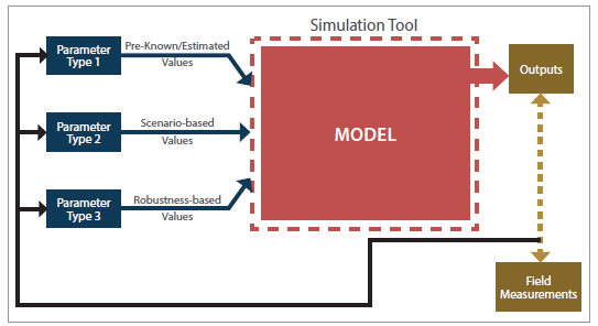
The limited degree of confidence decision criterion (Sldc) is a criterion where the indicator value is a weighted average of the weighted average indicator value and the minimax regret indicator value. This criterion implies the decision-maker’s degree-of-confidence in the probability distributions of the assumed scenarios. The degree-of-confidence is quantified using an appropriate weight. Figure 15 shows the robustness-based value generation procedure which is similar to the scenario-based value generation except that the robustness-based value generation includes a larger number of scenarios. Furthermore, evaluation of the robust sensitivity indicator is the key component that determines the selected scenario (values and probabilistic distributions for type 3 parameters). The overall framework, shown in figure 16, represents the simultaneity of entering different types of data into the traffic simulation tool.
Source: FHWA, 2019.
Figure 15. Illustration. Parameters with the deep uncertainty [type 3].
Source: FHWA, 2019.
Figure 16. Flowchart. Overall framework.
CONCLUSIONS
Vehicle trajectories provide the most complete record of a vehicle’s behavior over space and time, and afford the analyst the most flexibility and richness in characterizing virtually all aspects of traveler behavior and traffic system performance. Trajectories provide a unifying framework for conducting model calibration and subsequent validation of large-scale traffic operational models.
As noted, vehicle trajectories are still not regularly available to traffic analysts, though the situation is rapidly changing with greater willingness by system integrators and data vendors to share this information (albeit with all kinds of limitations on use). However, greater deployment of connected vehicle systems promises to dramatically increase the availability and accuracy of this type of data. From the standpoint of this project, in addition to possible sources of actual trajectory data to support the calibration framework development and application, a useful strategy would be to use simulated trajectories, i.e., the output of simulation models, as a way to develop and test the main calibration concepts and frameworks under development. An important advantage lies in the ability to then obtain measurements on the complete population of drivers in the network, allowing us the ability to test different partial observation scenarios (sampling schemes) on the accuracy of the results.