CHAPTER 2. REVIEW OF CALIBRATION METHODOLOGIES
Note: Unless accompanied by a citation to statute or regulations, the practices, methodologies, and specifications discussed below are not required under Federal law or regulations.
States are calibrating their traffic analysis tools to existing conditions, and then using those same calibration settings with future projected demand volumes to predict future performance. This practice is reflected in the state-specific modeling and simulation informational manuals published by various states. Moreover, there is little apparent variance in the calibration approaches when analyzing emerging technologies (e.g., advanced transportation demand management, integrated corridor management, connected and automated vehicles). As discussed in the first chapter, future conditions incorporate improvements that are significantly different than the base condition modeled when the analysis tool was calibrated. This can inhibit accuracy of the performance outcomes.
In recent years, there has been a growing interest in developing frameworks for calibration procedures that could be applied to different spatiotemporal settings. Such developments require a thorough understanding of the fundamental concepts underlying model calibration, as well as related validation principles. Calibration and validation procedures have tended to vary widely in practice, reflecting variation in available data and resources, as well as in the purpose of the motivating applications. In addition, there appears to be little consensus in the published literature and consultant informational documents regarding concepts, methods and best practice, including appropriate measures of effectiveness and calibration metrics. Many academic efforts have been devoted to modifying the optimization-based methods used for performing the calibration. As a result, the literature still lacks a systematic approach for calibration (So, et al. 2016)
Wegmann and Everett (2012) mentioned that the even the meaning of “calibration” and “validation” have changed over time, especially where funding limitations preclude the possibility of conducting travel surveys (for planning models) and/or taking needed measurements (for operational models). Under such limitations, default values are used for the model parameters in lieu of calibration using local data. Furthermore, lack of an independent database results in the calibration and validation processes becoming a single task. They provided information for calibrating each step of the transportation four-step model. For each step, they provided a list of measures along with candidate values and thresholds that could be used to evaluate the model.
As another attempt in this area, the MULTITUDE (Methods and tools for supporting the Use caLibration and validaTIon of Traffic simUlation moDEls) project, funded by the European Commission, has mainly focused on calibration methodologies and tried to bridge the gap between academic research and industry practice. According to a survey conducted in 2011 by Brackstone et al. (2012) among practitioners in the transportation industry, 19 percent of the respondents performed no calibration on the models that they developed and used. Moreover, among all those who performed the calibration process, only 55 percent followed sample steps provided in an informational manual instead of personal experience. Another finding is that calibration and validation have received more attention in the travel demand modeling area than the traffic flow simulation area.
The MULTITUDE document discusses several issues related to performing traffic simulation projects, including calibration:
- Definition of calibration.
- Structuring a simulation calibration activity.
- Calibration methodologies.
- Sensitivity analysis and the way to perform it.
- "Fall-back strategies" when calibration data are not available, and data transferability over various calibrations.
- Effect of model parameters considered in the calibration.
There have been numerous studies on the calibration of traffic simulation models. These studies differ from one another in different aspects including choice of algorithm, metrics used to compare the field-collected data and simulation model results, objective function utilized throughout the calibration process, parameters selected to calibrate, and choice of software.
Calibration of microscopic traffic behavior model parameters poses special challenges related to the difficulty of obtaining closed form expressions of the objective functions typically maximized or minimized in commonly used estimation techniques, such as generalized least squares or maximum likelihood. Thus estimation typically requires use of simulation or other numerical techniques to evaluate the objective function in the context of the estimation process. Furthermore, the lack of closed form expressions often precludes establishing rigorous mathematical properties that ensure convergence and uniqueness of the solution. For this reason, a variety of search techniques such as metaheuristics have been used in connection with this problem. Several studies in the literature have focused on one or the other algorithm for this purpose. Among these, genetic algorithm (GA) and variants (Cheu, et al. 1998, Kim, Kim and Rilett 2005, Ma and Abdulhai 2002, Park and Qi 2005, Chiappone, et al. 2016, Menneni, Sun and Vortisch 2008) and simultaneous perturbation stochastic approximation (SPSA) (Paz, et al. 2015, Balakrishna, et al. 2007, Lee and Ozbay 2009) are widely used in the literature. Some studies also performed a comparison of the performance of different algorithms. For instance, Ma et al. (2007) performed a comparison of the SPSA, GA, and a trial-and- error iterative adjustment algorithm over a portion of the SR-99 corridor in Sacramento, California. The comparison showed faster convergence of the SPSA algorithm; however, the other two algorithms reached a more stable set of calibrated parameters. Unfortunately, it is difficult to generalize from one set of comparisons as the results of such techniques often depend on the characteristics of the specific data set and model forms used.
Due to the high dimensionality of the problem, multiple local optima might exist for the problem. Accordingly, since the algorithms used in the literature are heuristic methods, a global optimum solution could not be guaranteed. Therefore, the calibrated parameter set found for the same problem might be different when a different heuristic algorithm and a different starting parameter vector are used.
The common set of metrics used in the calibration procedure are based on comparing simulated values (with the estimated parameters) to the observed values of traffic volume/flow, speed, capacity, density/occupancy, travel time, and/or origin-destination (O-D) flow. All these quantities could be derived if there is enough information regarding the observed and simulated vehicle trajectories.
The following formulas are some of the fitness functions used as the objective function for calibrating the simulation models (Yu and Fan 2017).
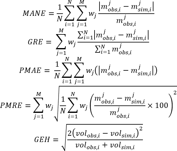
Figure 2. Formula. Fitness functions used as the objective function in calibration.
In figure 2 MANE is the mean absolute normalized error; GRE is the global relative error; PMAE is the point mean absolute error; PMRE is the point mean relative error; and GEH is a statistical measure named after Geoffrey E. Havers. Within the formulas, N is the total number of observations; M is the total number of measurements considered for comparing the simulation
results and the observations; mjobs,i(mjsim,i) denotes the ith sample value of the observed (simulated) metric j; volobs,i(volsim,i) represents the ith sample observed (simulated) traffic volume. Last but not least, wj is the weight assigned to each metric. Usually an equal weight is selected for each metric unless there is an inconsistency between the units of the components of the fitness function, such as the ones in the PMAE formula, or there is a situation that the researcher values one metric more than another. For instance, Paz et al. (2015) used a PMRE formulation for their objective function with different weights assigned to the link vehicle counts and link speeds.
So et al. (2016) presented a step-by-step approach for building, calibrating, and validating a microscopic model. In the calibration phase of their methodology, they first adjust the traffic flow descriptors (traffic counts, desired speed decisions, and reduced speed areas) and car-following parameters (maximum deceleration and acceleration rates, and minimum headway). Then the process goes through a calibration loop where the volume, speed, and travel time are checked sequentially based on their respective criteria. The modification of the model parameters are performed until the coefficient of determination for the turning movement traffic counts (R2) is more than 0.8 at all intersections. As the second step in the calibration process, the speed distributions on all links and the reduced speed areas in the simulation model are adjusted. Finally, the travel time is verified so that the R2 is more than 0.8 on all network sections. Since these three sequential steps might have a contradicting effect, a final calibration is performed considering all three goals simultaneously. Unfortunately, many values of the parameters to be calibrated could satisfy such aggregate criteria.
They tested the model on a large network consisting of 6 arterials and 160 intersections. This is one of the limited examples that a microsimulation calibration was performed on a relatively large network. One of the disadvantages of modeling such a large network is the high computational time required to develop and calibrate the model. Although they reached a significant accuracy in the calibration process, the validation process was only partially successful. They speculated that one of the reasons might be seasonal differences in the traffic demand distribution.
An innovation in the model calibration area is a software developed by Hale (2015) that has automated the calibration process to some extent. The software, with a published patent titled “System and Method for Automated Model Calibration, Sensitivity Analysis, and Optimization,” intends to make calibration a faster, cheaper, and easier procedure that requires less engineering expertise. Based on the software algorithm, the user selects the parameters and outputs for calibration as well as the level of calibration for each parameter. The software then performs the calibration and displays the field data metric, the simulated metrics, and the recommended values for each parameter. The software-assisted calibration architecture pertains to a simulation-based optimization category of simulation models. It contains a predefined narrow set of trial values for the input parameters. Similar to assigning a weight for each metric in other studies, the software is capable to prioritize the metrics evaluated in the objective function and the input parameters. Besides calibration, the software can be used to perform sensitivity analysis and solve a network optimization problem. Although the calibration process could conceivably be streamlined by deploying such software, the method has never been licensed to a commercial tool.
Hale et al. (2015) compared two optimization methods using the calibration software, namely directed brute force (DBF) and the aforementioned SPSA. They used CORSIM to model the I-95 corridor near Jacksonville, FL. The study period was divided into twelve 15-minute intervals. After calibrating the model using both optimization methods, they found that SPSA optimized the system more quickly. However, the effectiveness of SPSA relies on the suitability of the internal parameters and starting point. Moreover, the algorithm performs better when trial values are used instead of optimum (theta) values. Even with all these considerations, the SPSA algorithm usually provides local optimum solutions. On the other hand, the DBF algorithm would find the global optimum solution if the solution is within the user-defined search space. Furthermore, DBF is an appropriate algorithm for conducting sensitivity analysis. The authors concluded that a combination of the algorithms could be used to solve a calibration-related optimization problem. More specifically, the SPSA could be used to quickly find a local optimum solution then this solution could be fed as starting point to the DBF algorithm to locate the global optimum solution.
In summary, there have been many efforts in calibrating simulation models; these efforts share common elements in terms of the base model, the optimization algorithm, formulation of the objective function, etc., but differ in the specific choices made for these elements. One of the main limitations in existing studies is that the calibration process is based on available data, which mostly represent the normal prevailing condition of the transportation system. Some studies identified and specified additional scenarios developed on the basis of historical data. Offline calibration performed based on these datasets may not be robust enough to capture the future behavior of the system, especially when major changes are anticipated. Transferability of these models to future conditions of a system that might be subjected to fundamental changes in both demand and supply sides could be questioned. Furthermore, models that are calibrated online could only perform in a reactive manner. This reduces the effectiveness of the strategies suggested by the system when an anomaly occurs in the system that is not realized in the historical data under consideration.
Traffic is a complex system, and models developed to capture and predict its behavior often have many parameters that are estimated as part of the calibration process. Frequently, these parameters exhibit correlations across individuals, as they are intended to capture human behavior. Most of the previous studies performed the calibration procedure without considering the correlations that might exist between various parameters of a model. Ignoring these effects could result in solutions that are inconsistent with reality. Furthermore, as discussed later, considering these correlations, one could simplify the calibration process by reducing the dimensions of the pertinent optimization problem.
Different measures of effectiveness (MOE) have been selected in various studies presented in the literature. These are typically measured at fixed locations, and presented as aggregates over space and time. Calibration of microscopic behavioral models has often entailed specialized data collection with instrumented vehicles, or image processing of videos taken from fixed locations with limited visual field. An alternative that is gaining popularity is the use of vehicle trajectories (e.g., via Global Positioning System (GPS) tracking), which provide a comprehensive record of individual vehicle movement through a network. As such, trajectories could be used as an input from which various metrics/descriptors at various levels of detail could be extracted. Trajectories could be directly related to the demand parameters since they provide information regarding the origin and destination of a trip, though they do not convey information on other behavioral aspects associated with travel.
SCENARIO-BASED CALIBRATION
One of the approaches that would help calibration of transportation simulation models for anticipated/unexpected future conditions is a scenario-based simulation. There are many conditions that could impact a transportation system and induce variability in the model outputs. For example, major causes of variability in travel time could be traffic incidents, work zones, weather, special events, traffic control devices, demand fluctuations, and insufficient base capacity (J. Kim, H. Mahmassani and P. Vovsha, et al. 2013). Figure 4 shows a schematic of possible scenarios that might impact operation of a transportation network. It is essential to consider these sources of variability in the calibration process to develop robust models that could capture the relevant behavior of a transportation system.
Hou et al. (2013) developed a systematic procedure for calibration of a weather-sensitive Traffic Estimation and Prediction System (TrEPS). TrEPS is a tool that not only is able to capture the behavior of the system under different weather conditions, but can also implement weather- responsive strategies in the traffic management system. In the absence of relevant data, one can use the library of parameter values derived from TrEPS to construct some inputs of a dynamic network simulation model. This weather-sensitive system was integrated into a dynamic traffic assignment simulation framework, DYNASMART-P (DYnamic Network Assignment-Simulation Model for Advanced Road Telematics). The weather effect was formulated as a coefficient:
Figure 3. Formula. Weather effect coefficient in DYNASMART-P.
Where WAFi is the weather adjustment factor for parameter i, and fiweather event and finormal. represent the value of parameter i under a certain weather condition and under normal condition, respectively. After deriving the factor corresponding to each parameter, the factor is related to weather-related variables through a regression analysis. The coefficients of these regression models and the weather adjustment factors constitute a library that could be used in similar studies.
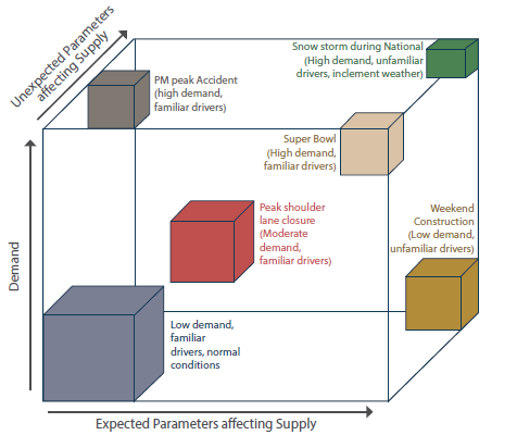
© Wunderlich, 2002.
Figure 4. Diagram. Schematic representation of different conditions that impact a transportation network.
The methodology was applied to the data collected for four metropolitan areas over several years to test the robustness of the methodology in calibrating a dual-regime modified Greenshields speed- density model under different weather conditions. Models developed for the case studies were calibrated through an iterative procedure that minimizes the root mean square error (RMSE) of speed. The results show that incorporating the weather adjustment factor in the model leads to a more realistic representation of the traffic conditions. In addition, a significant effect of visibility and precipitation intensity on some parameters of the fundamental diagram such as free flow speed and maximum flow rate was exhibited.
Kim et al. (2013) proposed a conceptual framework that uses commonly used traffic simulation models to capture the probabilistic nature of travel time. The framework is comprised of a scenario manager, a traffic simulation model, and a trajectory processor. The exogenous and endogenous sources of travel time variations are controlled respectively in the scenario manager component and in the traffic simulation model component. The last component of the framework processes the trajectories created by the simulator to measure the travel time for each scenario. This component also makes this study relevant to the trajectory-based calibration topic which is further discussed in the last section. The results of this framework could be translated into reliability measures for the urban network.
The methodology starts with determining the distribution of the demand and the equilibrium between demand and supply. Then, the scenario is specified for the distribution of scenario-specific parameters. The scenario is selected from the distribution of scenarios using a combination of the Monte Carlo and the mix-and-match approaches. After running the simulation model, the trajectories are developed. Then, the travel time distribution could be derived using the trajectories. Moreover, other reliability measures such as standard deviation of travel time, different percentile values of travel time, buffer index, misery index, planning time index, planning index, travel time index, and the probability of on-time arrival could be calculated using the vehicle trajectories. In order to calibrate the model for each scenario, an inner loop controls the demand-side scenario parameters and an outer loop adjusts the supply-demand equilibrium. The framework was tested on the data collected from 27.5 mi of the Long Island Expressway during the morning peak hours within a winter season. The results showed that the model parameters were consistent with the assumed scenario after the calibration procedure was performed.
Besides all the known sources of variability in transportation systems that might be reflected in historical data, there are conditions that have not been realized yet but are expected to be seen in the future. To improve the accuracy of the models in forecasting the network behavior under these situations, there is a need to generate these scenarios and develop reasonable probabilistic distributions for them.
Scenario-based approaches offer an important direction for making traffic models ready for a
variety of future conditions.
CORRELATED PARAMETERS
A possible source of error in previous calibration-related studies is that they did not consider the correlation between the parameters being estimated. Some studies investigated the effect of these correlations on the final results and proposed some methods to tackle this issue.
Kim and Mahmassani (2011) studied the effect of ignoring correlations among parameters when a
car-following model is calibrated. The authors selected three car-following models including the Gipps model, the Helly linear model, and the intelligent driver model (IDM). Six metrics were chosen to compare the effect of parameter correlation on different objective functions defined for the calibration procedure: network exit time, total travel time, mean of average spacing, the standard deviation of average spacing, mean of the coefficient of variation of spacing, and standard deviation of coefficient of variation of spacing. They evaluated the correlation effect using the Next Generation Simulation (NGSIM) trajectory data. First, the correlations between parameters of the dataset were studied using the factor analysis approach. To investigate the parameter correlation effect, they developed two sets of simulation models. One by sampling from the marginal distribution of the model parameters (ignoring the correlation effects) and the other by sampling from the joint distribution of the model parameters (preserving the correlation effects). Then, the models were calibrated by solving the optimization problem using the downhill simplex method. The distributions of the results were compared to the relevant distribution developed based on the NGSIM data using the Kolmogorov–Smirnov test. The comparison showed significant discrepancies between the result of the calibrated models that correctly considered parameter correlations and the calibrated models that ignored parameter correlations. As expected the results of the models that preserved the correlation effect were closer to the field data.
Prakash et al. (2018) suggested a generic calibration methodology to perform dynamic traffic assignment in real time. As mentioned earlier, one of the limitations associated with the state-of- the-art approaches in calibration is that they are spatially limited to a small network or they are applied to a limited set of parameters, incorporating both demand-side and supply-side parameters. The authors addressed these limitations by systematically reducing the dimension of the problem. They proposed a state-space formulation and solved the problem using the Constrained Extended Kalman Filter approach. In order to reduce the problem dimension, they performed a principal component analysis. The following formula shows the state-space formulation used for the generic online calibration problem:
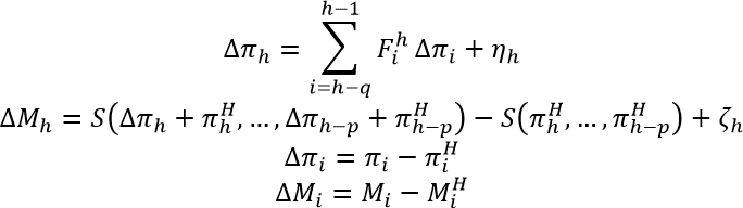
Figure 5. Formula. State-space formulation for generic online calibration.
Where πi (Mi) represents the model parameters (measurements) in the time interval i. On the other hand, πH(MH) contains the historical values of the parameters (measurements) in time interval i; ηh(ζh) is a vector of random errors in the transition (measurement) equation;  is a matrix that relates the parameter estimates of interval i to the estimates of interval h; S(.) denotes the simulation model; q is the degree of the autoregressive process; and p denotes the maximum number of previous time interval’s parameters which influence the current interval’s parameters.
The authors listed three main assumptions of the methodology as follows: using time-invariant principal component directions, the linearity of transition equation, and performing a sequential online calibration that neglects the effect of estimated parameters on the previous time intervals. However, these simplifying assumptions do not sacrifice the accuracy of the model significantly.
They applied the methodology to a large Expressway network in Singapore that constitutes 936 nodes, 1,157 links, 3,906 segments, and 4,121 O-D pairs. The time required for estimating the calibrated parameters of the model for such a large network based on this methodology was less than 5 minutes. Followed by the model calibration, they performed a sensitivity analysis to study the effect of the degree of dimensionality reduction on the accuracy of the model.
As mentioned previously, there are several ways to consider the correlation that might exist between parameters that are considered in the calibration procedure. Recognizing the correlation could help reduce the size of the problem and develop more reliable models. With the advent of new technologies and fundamental transitions in travel behavior, it is important to study the correlation between parameters that would be introduced to the transportation system and already existing parameters to improve the performance of simulation models.
TRAJECTORY-BASED CALIBRATION
Vehicle trajectories are becoming an increasingly available form of observation of individual traffic and traveler movement in networks, largely due to the prevalence of GPS-enabled cell phones and navigation systems in vehicles. Trajectories constitute records of vehicle presence at various points along a network.
Information that can be extracted from trajectory data includes (H. S. Mahmassani 2016):
- Time; i.e., position of this moment on the timescale.
- Position of the vehicle in space.
- Trip origins and destinations.
- Direction of the vehicle‘s movement.
- Speed of the movement.
- Dynamics of the speed (acceleration/deceleration).
- Accumulated travel time and distance.
- Individual path and temporal characteristics.
In addition, from groups of trajectories, the following could be obtained:
- Distribution of speed/travel time (for reliability analysis).
- Probe vehicle density.
- Inferred traffic volume.
Trajectories provide a more complete and compact description of system state than fixed sensors, as they capture all aspects of individual actions (most complete record of actual behavior), with no loss of ability to characterize systems at any desired level of spatial and temporal aggregation or disaggregation. Furthermore, they retain the ability to extract stochastic properties of both individual behaviors and performance metrics (Kim and Mahmassani 2015).
Trajectories are also a common output of particle-based (microscopic and mesoscopic) simulation tools is one of the model outputs that could be used to generate other system metrics at a different level of aggregation. The level of aggregation could vary from reflecting the performance of the system in a small segment of the road to summarizing the performance of the entire network in a single number (Saberi, et al. 2014). As a result, they enable better model formulation/specification at all levels of resolution, effectively unifying model calibration and network performance analysis.
Trajectories have played a key role in the calibration of microscopic models of car following (Hamdar, et al. 2008) and lane changing (Talebpour, Mahmassani and Hamdar, 2015). Ossen and Hoogendoorn (2008) mentioned that calibration of car-following models could be impacted by methodological issues, practical issues related to the use of field data, and measurement errors.
The authors investigated the effect of measurement error on calibration results. To grasp a better understanding of this effect, they introduced several types of measurement errors to a synthetic dataset. They simulated the trajectory of the follower based on the given trajectory of the leader and a selected set of parameters using the Gipps model and the Tampere models. As the first step, they used the Bosch trajectory data collected in Germany as the leading car trajectory and then produced a clean synthetic dataset for the following car based on each car-following model and random sets of model parameters with uniform distribution. In the second step, the errors were incorporated in the leading car and following car datasets considering a variety of statistical distributions. Several statistical distributions were used to accommodate the effect of error magnitude, systematic errors, and nonsymmetrical errors. The calibration was performed in the next step by minimizing two separate objective functions: one based on vehicle speed and the other based on headway. The problems were solved using the simplex method. They found that in addition to the significant biases caused by measurement errors, the optimization problem could generate results that contradict the car-following behavior. Another problem caused by these errors is the reduction in sensitivity of the objective function and reliability of the results. The authors suggested smoothing the data by the moving average method to alleviate some these issues.
As a result, the vehicle trajectories as mentioned earlier are very useful in calibration of simulation models. However, due to the large effect of small errors introduced in the models that generate vehicle trajectories, care should be exercised in such analyses.
CONCLUSIONS
States are calibrating their traffic analysis tools to existing conditions, and then using those same calibration settings with future projected demand volumes to predict future performance. Unfortunately, because future conditions incorporate improvements that are significantly different than the base condition modeled, this can inhibit accuracy of the performance outcomes.
Significant research into calibration of traffic analysis tools has taken place in recent years. Thanks to these studies, we have learned more about the potential effectiveness of certain heuristic methods (e.g., genetic algorithm) and fitness functions (e.g., RMSE). However, these studies have not addressed the challenge of developing robust models for future conditions.
Other research avenues appear more promising for informing an overall methodology or framework for modeling future conditions. One of these is a scenario-based simulation. To improve the accuracy of models in forecasting network behavior under various situations, there is a need to generate scenarios and develop reasonable probabilistic distributions for them. Secondly, a possible source of error in previous studies is that they did not consider parameter correlation. There are several ways to consider the correlation that might exist between parameters considered in the calibration procedure. Recognizing this correlation could help reduce the size of the problem, and develop more reliable models. Lastly, the use of vehicle trajectories is gaining popularity. Trajectories provide a more complete description of system state. They retain the ability to extract stochastic properties of both individual behaviors and performance metrics. Trajectories could be directly related to the demand parameters, though they do not convey information on other behavioral aspects associated with travel.