Decision Support Framework and Parameters for Dynamic Part-Time Shoulder Use:
Considerations for Opening Freeway Shoulders for Travel as a Traffic Management Strategy
Appendix C. Decision Parameter Development Methods
This appendix provides technical details to supplement chapter 4 and provides additional information on two decision parameter methods discussed in chapter 4.
B1. Breakdown Probability Estimation with Method II — Emperical Performance Data
An empirical approach is adapted from the literature, (Brilon, Geistefeldt, & Regler, 2005) which identifies the probability of traffic flow breakdown based on the assumption that capacity is intrinsically stochastic. The method is based on the statistics of censored data. It delivers an estimation of the capacity distribution function Fc(q), representing the probability of a traffic breakdown in dependence on the flow rate q:
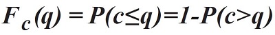
Figure 54. Equation. The capacity distribution function.
where:
Fc(q) is the capacity distribution function, representing the breakdown probability at traffic volume q.
q is the traffic volume in vehicles per hour per lane (veh/h/ln).
c is the capacity (veh/h/ln), i.e., the traffic volume beyond which traffic flow will break down into congested conditions.
P(c>q) is the probability that the capacity is greater than the observed volume.
In the light of the difficulty in selecting an appropriate fixed value for capacity, one could select values based on a "tolerable probability of breakdown." (Elefteriadou, 2014)
Traffic flow observations deliver pairs of average speeds and volumes in selected time intervals (e.g., 5 minutes). In intervals prior to a traffic breakdown that results in a speed drop below a specified threshold speed in the next time interval, capacity can be measured directly. In intervals not followed by a breakdown, capacity must have been greater than the observed volume. These observations are called "censored" observations. To estimate distribution functions based on samples that include censored data, both non-parametric and parametric methods can be used.
A non-parametric method to estimate the distribution function of lifetime variables is the product limit method (PLM). (Elefteriadou, et al., 2009) The PLM is based on work by Kaplan and Meier, which uses lifetime data analysis techniques for estimating the time until failure of mechanical parts or the duration of human life (Kaplan & Meier, 1958). Brilon et al. (2005) used this method in the context of freeway breakdown to estimate the capacity in a true stochastic sense. The productlimit estimator for the capacity or breakdown probability distribution is given by:
Figure 55. Equation. The product-limit estimator for the capacity or breakdown probability distribution. (Elefteriadou, 2014)
where:
q is the traffic volume (veh/h/ln).
qi is the traffic volume in interval i.
P(qi>q) is the probability that the observed breakdown volume is greater than the observed volume.
The product-limit estimator for the probability of observed breakdown volume being greater than the observed volume is given by:
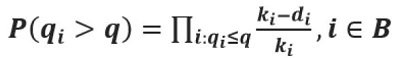
Figure 56. Equation. The product-limit estimator for the probability of observed breakdown volume being greater than the observed volume.
where:
q is the observed traffic volume (veh/h/ln).
qi is the observed traffic volume at interval i, which is the one prior to the drop in speeds; i.e., defined as the observed breakdown flow (veh/h/ln).
ki is the number of intervals with a traffic volume of q≥qi.
di is the number of breakdowns at a volume of qi.
B is the set of breakdown intervals {B1,B2,…}.
However, if each observed volume that causes a breakdown is considered separately; i.e., only one observation of breakdown for every volume qi ; di = 1, then the product-limit estimator is given by:
Figure 57. Equation. Product-limit estimator for observed volume that causes a breakdown but is considered separately.
with all the terms defined as previously.
For a parametric estimation of the breakdown probability distribution, the function type of the distribution must be predetermined. The distribution parameters can be estimated by applying the maximum likelihood technique. For capacity analysis, the likelihood function is:
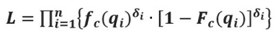
Figure 58. Equation. The likelihood function for capacity analysis.
where:
fc(qi) is the statistical density function of the capacity c.
Fc(qi) is the cumulative distribution function of the capacity c.
n is the number of intervals.
δI = 1, if interval i contains an uncensored value.
δI = 0, if interval i contains a censored value.
To simplify the computation, it is useful to maximize the log-likelihood function instead of the likelihood function L.
Calculating the breakdown probability distribution will provide agencies with guidance on observing and measuring (1) maximum pre-breakdown throughput, and (2) breakdown flow at the agencies' desirable probability of breakdown value.
Agencies with new dynamic part-time shoulder use (D-PTSU) facilities, including conversions from static part-time shoulder use (S-PTSU), may want to open the shoulder less frequently and be more tolerant of congestion. Agencies more experienced with D-PTSU may want to be more aggressive opening the shoulder and do so even with a lower probability of congestion if it were not opened.
B2. FREEVAL Modifications to Support D-PTSU Analysis with Method III — Macroscopic Decision Parameter Optimization
The computational procedure in the Highway Capacity Manual (HCM) freeway facilities methodology is defined in terms of two distinct operational regimes. The first regime handles conditions where all segments are operating under capacity and is referred to as the "undersaturated" method. The second applies when at least one segment is operating over capacity or at level of service (LOS) F and is referred to as the "oversaturated" method.
The undersaturated method provides operational analysis in 15-minute increments. This increment is fixed as required by the set of underlying regressions on which the method is based. Alternatively, the oversaturated method is based on the cell transmission model, an approach which allows time steps of any length. The HCM fixes the oversaturated computational time step length at 15 seconds in accordance with certain assumptions of the methodology. Further, in order not to overwhelm users with extensive outputs, but to provide consistency within the undersaturated approach, the analysis using the oversaturated method is always aggregated up to the same 15-minute resolution as the undersaturated methods.
In the context of this project, there are two primary considerations relating to the use of the HCM method. First, the analysis is focused on operational conditions where demand is likely to exceed capacity and result in a breakdown that the PTSU strategy will attempt to mitigate or even eliminate. Since congested conditions are those of primary interest, it is assumed that the oversaturated method will be used for the entirety of the analysis. While it does not provide the exact same operational results as the individual segment methodologies during undersaturated time periods, the oversaturated approach does adequately approximate the method to the extent that it will not demonstrably affect the results of the experiment.
The second consideration is that the default 15-minute time step provides an analysis resolution that is too coarse to capture the necessary responsiveness of a D-PTSU system. However, as mentioned previously, the oversaturated approach actually updates operational conditions at a 15-second resolution before being aggregated to 15-minute results for consistency. By overriding the HCM's default 15-minute aggregation of results and replacing it with a reduced increment, such as a oneminute resolution, this issue can be circumvented in a straightforward manner without any true modifications to the methodology.
Bypassing the 15-minute aggregation of results does not require changing any underlying methodological assumptions or modifying any specific computational steps. Rather, it is accomplished by changing a single global variable of the methodology as defined in chapter 25 of the HCM: S — the number of computational time steps in an analysis period.
Reducing this from the default value of 60 (corresponding to a 15-minute analysis period) to a value of 4 effectively sets the length of an analysis period of the methodology to one minute. This required modification to the aggregation procedure as well as corresponding updates to the interface, which were made directly within the open-source FREEVAL engine to support the computational details needed for this project and the effective modeling of D-PTSU.