Behavioral/Agent-Based Supply Chain Modeling Research Synthesis and Guide

CHAPTER 4. AGENCY EXPERIENCES WITH BEHAVIORAL/AGENT-BASED SUPPLY CHAIN MODELS

This chapter details the comprehensive review of the state-of-the-practice models. The models reviewed are summarized along 12 dimensions related to methodology and data. The information in this chapter is based on the information collected and reviewed from the public agencies identified in Chapter 1. Models are presented in order of development date, from earliest to most recent.

CHICAGO METROPOLITAN AGENCY FOR PLANNING

Methodology

The Chicago Metropolitan Agency for Planning (CMAP)¹ has been incrementally building a regional freight model since 2010. CMAP first developed the firm synthesis, supplier selection, and mode choice elements of its freight modeling system (Cambridge Systematics, 2011). CMAP then added supply chain and logistics elements and truck-touring models (RSG, University of Illinois at Chicago and John Bowman, 2012). Finally, CMAP (RSG, 2017) developed an extension to the mesoscale model, a modeling tool for forecasting future freight flows under different sets of investment, policy, and macroeconomic scenarios. The mesoscale model extension can help analyze industries and answer questions regarding how such industries might affect the freight-dependent business community.

Supply Chain Modeling Needs

CMAP developed a freight forecasting model for policy and planning sensitivity analysis to systematically vary forecasts to reflect potential changes in macroeconomic conditions (e.g., foreign trade levels, price of crude oil); large-scale infrastructure changes (e.g., port expansions, new intermodal terminals); technological shifts in logistics and supply chain practices (e.g., near-sourcing, outsourcing, productivity enhancements); and other assumptions and scenario inputs related to the economic competitiveness of the Chicago region and its infrastructure investments. CMAP also intends to use their freight forecasting model to evaluate performance of local freight facilities (e.g., transfer terminals, roads, rail, water, and air cargo infrastructure). The Chicago region's long-range comprehensive plan calls for the development of robust modeling tools to address the local and regional effects of freight transportation-based changes in the economy and freight delivery systems. CMAP desires an analysis tool that explains the economic choices made for goods movement across multiple modes and commodities, and that provides a picture of the region's role in the national freight economy. Once the updated model (currently under development) is ready to use, initial efforts will focus on providing an understanding of how freight currently moves throughout the region. As a start, CMAP freight planning staff may be interested in evaluating the regional impacts of freight policies such as overnight delivery ordinances or the expansion of logistics terminals within the region.

Model Structure, Component Interactions, and Segmentation

The national-scale portion of the CMAP freight model addresses how establishments that buy goods select suppliers and how suppliers ship goods to their buyers. Figure 12 presents the CMAP national-scale model structure process.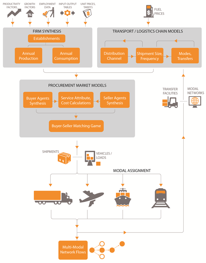

Figure 12. CMAP National-Scale Supply Chain Model Process.
Source: (RSG, 2017)

Initially, the model synthesizes establishments across the United States by industry and size category. The model then determines the complexity of the distribution channel used in the supply chain. Multinomial logit choice models determine the supply chain type based on buyer-supplier pair characteristics and industry characteristics. The four chosen distribution channels represent complex supply chains rather than a single supply chain.

The national-scale models identify the shipment size, frequency, and mode of shipments based on travel time and cost and the characteristics of the shipments and distribution channels.

CMAP uses a flexible agent-based computational economics approach for modeling the evolution of regional supply chains, as influenced by key economic drivers. The model starts by synthesizing U.S. establishments by industry classification and size, locating them spatially, and deriving annual production and consumption requirements from existing commodity flow relationships between producing and consuming sectors of the national economy, as represented in U.S. Bureau of Economic Analysis benchmark IO accounts data. The model system also synthesizes agents representing establishments in countries and industries that currently trade with the United States.

For each commodity market, an iterative procurement market game (PMG) is played. The PMG involves a pool of buyers who attempt to procure inputs from a pool of sellers in the market. As an input to the PMG, the transport-logistics chain models simulate the choice of distribution channels, shipment sizes, and modes for each prospective buyer-supplier pair, thereby enabling the calculation of logistics costs and shipping times. Buyers consider shipping times, unit costs (transport and nontransport), and risk minimization (e.g., supply chain disruption). Sellers, who are capacity constrained, evaluate whether to trade with a buyer in the face of other, potentially more lucrative offers. Through repeated bilateral games, agents form preferences for specific trading partners based on past interactions and may adjust their tolerances for risk based on market constraints.

The final round of the game (after a user-specified number of iterations) indicates which agents established trading relationships and the quantities of commodities bought and sold, producing a set of spatially distributed freight flows between establishments located in freight analysis zones. In most markets, buyers will far outnumber sellers; however, buyers will likely purchase commodities from multiple sellers, either for risk-minimization reasons or limited individual seller capacity. Because foreign buyers and sellers are included in the procurement market, the model also predicts import and export flows.

The regional-scale truck-touring models were developed as integrated elements of the freight modeling system, with direct inputs from the national-scale supply chain models. The model produces trip lists for all the freight delivery trucks in the region that can then be assigned to a transportation network. The truck-touring model components predict the elements of the pick-up and delivery system within the Chicago region through several modeling components, as shown in Figure 13:

• Vehicle and tour pattern choice. Predicts the joint choice of whether a shipment will be delivered on a direct- or a multi-stop tour and the size of the vehicle that will make the delivery.
• Number of tours and stops. Predicts the number of multi-stop tours required to complete all deliveries and estimates the number of shipments that the same truck can deliver.
• Stop sequence and duration. Sequences the stops in a reasonably efficient (but not necessarily the shortest-path) sequence. Predicts the amount of time taken at each stop based on the size and commodity of the shipment.
• Delivery time of day. Predicts the departure time of the truck at the beginning of the tour and for each subsequent trip on the tour.

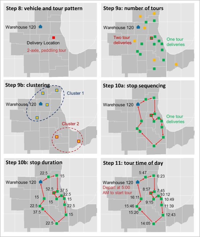
Figure 13. CMAP Regional-Scale Truck-Touring Model Process.
Source: (Smith, 2013)

The model simulates the evolution of globally connected supply chain relationships in the Chicago region and how these trading relationships translate to regional freight flows defined by industry, commodity, size, and mode. The buyer-supplier matching component operates as a processing kernel within the larger mesoscale freight model to simulate the evolution of supply chain relationships, rather than allocating a fixed freight demand. The regional tour-based truck model component evaluates the performance of existing and future regional freight facilities.

Market Segmentation (Industry, Commodity, Mode, Vehicle Type, Temporal, Activity Type)

The CMAP freight model employs several types of market segmentation depending on the unit of analysis of each model component:

• Represents 20 industry categories and seven establishment sizes in employment data, resulting in 140 classifications of establishments, by size.
• Represents 43 Standard Classification of Transported Goods (SCTG) commodity groups.
• Includes four primary modes (i.e., road, rail, air, and water) in the mode choice model.
• Includes three types of trucks (light, medium, and heavy) in the vehicle choice and tour pattern model.
• Estimates freight tonnages annually and then converts truck tonnages to average daily tonnages. Simulates truck deliveries by the minute and aggregates to the CMAP regional time periods for assignment.
• Identifies truck deliveries as pick-up or drop-off. Includes no service-related truck tours or intermediate stops for driver meals, gas refills, or breaks.

Assumptions Made Regarding Agent/Behavioral Relationships

The model makes various assumptions regarding inputs to the model and relationships between buyer and seller agents. For example, in the PMG kernel, some input parameters reflect different assumptions regarding buyer tradeoffs between supplier cost and responsiveness and risk hedging. In addition, different sets of parameters and payoff weights are specified in the model to reflect assumed information available to agents and whether market prices are static or adjusted throughout game play. In general, PMG behavioral parameters reflect assumptions about the possible mindsets of buying and selling agents as they seek out and try to secure favorable procurement contracts for their establishments. The CMAP model recommends a baseline set of PMG parameters, motivated by the aspiration to represent plausible agent behavior under the following assumptions:

• Agents do not have perfect information about all agents in the market, but do have information about the agents with whom they have had trading encounters and know both their own rating of past trades and how their trading partners rated them.
• Agents learn through successive iterations, accumulating experiences, and updating their knowledge about agents with whom they have new trading encounters.
• Both buyers and sellers evaluate the potential for future trades with each other using weighted payoff values that consider the perceived strength of trading relationships, as opposed to pure cost minimization or revenue maximization.
• The commodity market under study is in a steady state, and agents are price-takers who do not affect average commodity prices in the short term.
• It is unknown whether buyers are of the type who tend to satisfice quickly and stick with their initial trading partners, or are of the type who are inclined to seek out potentially new and better trading partners.

Also, for import/exports of commodities, it is assumed that the amount produced by each country for a commodity represents a fixed production capacity (supply), and ignores the demand-supply impacts of sales to non-U.S. countries. Similarly, the model assumes that the amount that the United States exports to each country represents a fixed demand for U.S. goods and ignores the demand-supply effects of purchases from non-U.S. countries.

Modeled Performance Measures

• Models annual tonnage shipped by mode to, from, and through the Chicago region.
• Models cost per ton of freight shipped, by mode.
• Models market share of international or regional trade.
• Models origin-destination (O-D) travel times, by mode and commodity.
• Models daily trucks, by time period and road segment.

Approach to Forecasting

The CMAP freight model is run as a standalone scenario (currently only a base year exists) through RStudio software. The truck-touring component of the freight model outputs a set of time-of-day truck trips in CMAP's modeling zone system that can serve as inputs to the regional trip-based model in place of the current truck demand used within the model. CMAP has verified that this functionality works but has not yet used freight model truck trip tables for any planning analysis. CMAP has not developed any actual scenarios for the PMG version of the freight model. A consultant contract is underway that will develop and test at least one alternative scenario for sensitivity testing purposes. This work will include the development of methods and procedures to modify input data as appropriate.

Types of Applications and Procedures

The current freight model is still in the development phase and has not been used for any planning analysis. The current consultant contract will calibrate the mode choice component of the freight model and will validate the model's output commodity flows. CMAP staff will begin to use the model for planning analyses after this work is completed (anticipated by the end of 2017). To date, CMAP has applied this system to a limited set of sensitivity tests (constrained to varying the PMG input parameters for a set of selected commodity markets).

Data

Geographic Scope

The CMAP freight model has multiple levels of resolution and can forecast freight flows between Chicago and the rest of the world (mesoscale). It also includes an intraregional truck-touring model (microscale). The different systems (meso and micro) are used for apportioning high-level commodity flows to individual shipper-receiver pairs and identifying the set of feasible transport paths for each shipper-receiver pair:

• National and International Zones. Comprises domestic FAF4 zones and international FAF4 zones in broadest zone system. It is used for the FAF4 commodity flow input data. International zones include eight international regions used for imports and exports.
• Statewide Traffic Analysis Zones (TAZs). Comprises traffic analysis zones that are smaller in size (within Chicago Urban Area and surrounding area of Illinois, Indiana, and Wisconsin) with subcounty-size TAZs (Figure 14) in mid-level zone system. This zone system is used during the establishment allocation and modes and transfers steps.
• Regional TAZs. Comprises TAZs that are smaller than statewide zones, but larger than passenger model zones (Figure 15) in the regional zone system. This zone system is used for all the truck-touring model components.

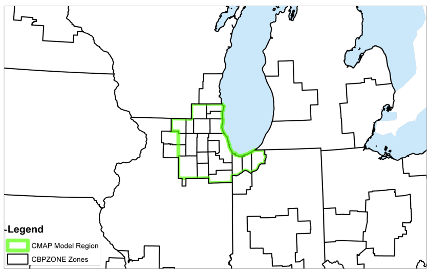
Figure 14. CMAP Statewide TAZs.
Source: (Cambridge Systematics, 2011)

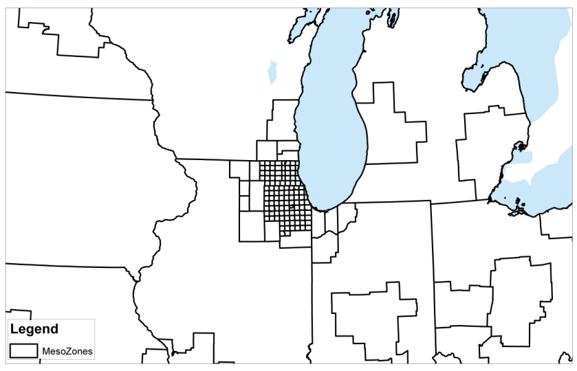
Figure 15. CMAP Regional TAZs.
Source: (Cambridge Systematics, 2011)

Data Inputs

The CMAP freight model uses the following data sources as data inputs:

• Zone Systems. Freight Analysis Framework (FAF) zone system (FHWA), county-level zone system (U.S. Census Bureau), and CMAP mesoscale zones.
• Economic Data. Input-Output (IO) Make and Use tables (BEA) and industry to commodity correspondences (BEA and Freight Activity Microsimulation Estimator [FAME]).
• Employment Data. County Business Patterns (CBP) data (U.S. Census Bureau) and CMAP employment data.
• USA Census Trade Online. Volumes of imports and exports of commodities flowing to and from the United States and other countries.
• Networks. Uses CMAP's mesoscale model freight network to derive skims. The model uses detailed networks of road and rail in the United States, but estimates detailed networks of air and water using simple functions of distance and the value of goods being transported.

Data Used for Estimating Model Parameters

The CMAP freight model uses the following main data sources for estimating model parameters:

• Data collected for a national survey as part of the FAME project (Samimi A. M., 2010). Uses these data to identify four distribution channels comprising combinations of intermodal terminals, warehouses, consolidation centers, and distribution centers (i.e., direct shipments, one type of intermediate stop, two types of intermediate stops, or three or more types of intermediate stops).
• Commercial vehicle surveys collected in Texas. Uses these data to predict shipment weight and number of shipments per year.
• Research conducted by de Jong and Ben-Akiva (de Jong, 2007). Adapts this research to use in the mode and intermediate transfer model to predict the mode and path of long-haul movements of freight based on a comprehensive accounting of transport and logistics costs.

Data Used for Model Calibration

Under the new model update contract, CMAP expects to calibrate the mode choice model used to estimate shippers' choices. This is anticipated to be accomplished by comparing the freight model-derived modal shares used to transport significant commodities or commodity groups within the national economy to modal shares reported by other data sources. These data sources may include (but are not limited to) the FAF data, the Public Use Waybill Sample, Waterborne Commerce Statistics Center data, and the 2012 Commodity Flow Survey (CFS) Public Use Microdata (PUM) file.

Data Used for Model Validation

CMAP plans to validate the PMG portion of the model against observed commodity flows (e.g., FAF data) as part of the new model update work. Two types of validation will involve comparisons with observed data where data are available, and in cases where data are not available, a process validation compares the outcomes of the model with anticipated outcomes based on the mathematical algorithm that the model is intended to simulate. The validation will examine several outputs from the firm synthesis and procurement market models that collectively lead to the shipment flow outputs produced by the model (e.g., location and magnitude of commodity production and consumption, spatial commodity flow patterns, and magnitude of commodity flows). The validation process design will depend on identifying what data are available to support validation. The geographic scale achievable using the FAF data is likely limited to FAF zone to FAF zone, which is essentially State or major metro area to State or major metro area. The validation task will likely rely on a similar set of datasets to those used to calibrate the mode choice model.

Data Desired, but not Found

Some of the desired—but unobtainable—data for use in the model included the following:

• Data for estimating logistics costs calculations (e.g., storage costs, warehouse handling charge).
• Data for maximum load weight of truck types in the vehicle tour choice pattern component of the model.

Detailed information about the model and the freight datasets is not yet available online.

FLORIDA STATEWIDE

Methodology

The Florida Department of Transportation's Freight Supply Chain Intermodal Model (FreightSIM) (RSG, 2015) is a travel demand model component integrated into the Florida Statewide Model (FLSWM). FreightSIM simulates the transport of freight between supplier and buyer businesses in the United States, focusing on Florida-specific movements. FreightSIM produces a list of commodity shipments by mode and converts those to daily truck trip tables that can be assigned to the national and statewide networks in the FLSWM along with trip tables from the passenger model. The approach used in the development of FreightSIM employs supply chain and economic methods to explicitly model aspects of freight decision-making behavior. The model is intended to provide decision-makers with better information to make decisions about transportation investments and policies. The supply chain methods at a national scale in this framework have been adapted to include additional level of detail (zone system) in Florida.

Supply Chain Modeling Needs

Providing freight mobility in a cost-effective manner requires an understanding of supply chain and logistics behavior and an evaluation of investments in transportation infrastructure and services. It also requires anticipating the effects of any government and private sector decisions that affect the transportation system and its uses. The development of a multimodal supply chain shipment model was focused on addressing this overall objective. Trends affecting freight mobility in Florida over the next 50 years include an innovation economy with emerging mega-regions and industries such as aerospace, clean energy, life sciences and creative industries; shifting global markets and development patterns; new communication technologies and environmental stewardship challenges; and the changing role of the public and private sectors (Florida Department of Transportation, 2010). Challenges for the transportation system arising from these trends include: efficient and reliable connectivity as a global hub, congestion on intercity corridors, new logistics practices, sustainable environmental practices, and available funding.

A multimodal supply chain shipment model of goods movement for Florida was developed to assist with the following:

• Inform infrastructure investment decisions.
• Evaluate congestion on Florida's highways.
• Test the effectiveness of statewide transportation policies on mobility and the economy.
• Produce multimodal system performance measures for freight.
• Evaluate the effects of private sector decisions on the State transportation system.
• Provide regional agencies with intercity freight travel for regional planning purposes.

The goal for FreightSIM is to account for changes to freight mobility based on these types of policies.

Model Structure, Component Interactions, and Segmentation

FreightSIM simulates the transport of freight between each supplier and buyer business in the United States. Figure 16 illustrates these processes and identifies major input and output data. This modeling system includes the selection of business locations and trading relationships between businesses; it also includes the resulting commodity flows, distribution channel, shipment size, and mode and path choices for each shipment made annually:

• Firm Synthesis. Synthesizes all establishments in the United States and a sample of international establishments.
• Supplier Firm Selection. Selects supplier establishments for each buyer establishment, by type.
• Goods Demand. Predicts the annual demand (in tonnage) for shipments of each commodity type between each establishment in the United States.
• Firm Allocation. Allocates firms in each county to TAZs within the Florida region (including Georgia and Alabama).
• Distribution Channels. Predicts the level of complexity of the supply chain (e.g., whether it is shipped directly or whether it passes through one or more warehouses, intermodal centers, distribution centers, or consolidation centers).
• Shipment Size and Frequency. Estimates discrete shipments delivered from the supplier to the buyer.
• Modes and Transfers. Predicts four primary modes (road, rail, air, and waterway) and transfer locations for shipments with complex supply chains.
• Trip Assignment. Assigns shipments to specific warehouse, distribution, and consolidation centers if the shipment passes through one of those locations, and predicts truck and auto volumes on the highway network.

The model incorporates a multimodal transportation network that provides supply side information to the model, including costs for different paths by different modes (or combinations of modes). The model encompasses all of Florida and freight flows between Florida and the rest of the world. Truck flows are assigned with passenger trip tables to highway networks to produce auto and truck volumes across the United States. The validation data are for rail, air, and waterway flows and these data are retained as trip tables instead of being assigned.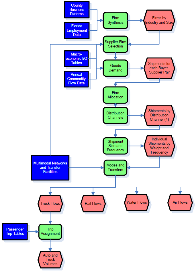

Figure 16. CMAP Regional-Scale Truck-Touring Model Process.
Source: (RSG, 2015)

Market Segmentation (Industry, Commodity, Mode, Vehicle Type, Temporal, Activity Type)

FreightSIM employs several different types of market segmentation depending on the unit of analysis of each model component. The firm synthesis model characterizes business establishments by location (TAZ), establishment size (eight employment categories ranging from 1–19 employees to over 5,000 employees), and industry (six-digit Census Bureau NAICS categories). The firm synthesis model is controlled at the TAZ level within Florida using the statewide employment forecast data. The employment forecasts are grouped into three employment categories that are aggregations of NAICS categories. The commodity production and consumption by business establishment uses the BEA's six-digit NAICS categories, which is slightly aggregated in comparison to the U.S. Census Bureau's NAICS categories used for the industrial classification of the business establishments.

The supply chain model works with FAF commodity flow data and uses the 43 SCTG categories for segmentation of shipment commodity. The distribution channel of the shipment flow through the supply chain is segmented into direct shipments using one, two, or three transfers at distribution centers or intermodal transshipment locations. The supply chain model allocates shipments into size categories using a two-stage process, ultimately calibrating the distribution to the nine shipment-size categories, ranging from less than 50 pounds to more the 100,000 pounds used by the CFS. The shipments are allocated to one of four main modes (i.e., truck, rail, water, or air), with the intermodal paths being some combination of those modes (e.g., truck-rail-truck). The conversion to trip tables of the outputs from the supply chain model uses truck percentages for light, medium, and heavy trucks (FHWA classes 2–3, 4–7, and 8–13, respectively). The trip tables are divided into four time-specific trip tables (AM peak, midday off-peak, PM peak, and nighttime off-peak) using fixed factors.

Modeled Performance Measures

FreightSIM includes the following performance measures:

• Models shipment size and weights, by commodity.
• Models truck, rail, air, and water trips, by district.
• Models annual import and export flows, by port.
• Models daily truck volumes, by district, area type, facility type, and screenline.
• Models daily truck travel times for select O-D pairs.

Approach to Forecasting

The freight demand, supply chain, and mode and transfer components of FreightSIM are run for each forecast year using the R open-source statistical programming platform and are integrated with the FLSWM that is implemented in the Cube software. The statewide model includes the following primary groups or steps:

• Building highway network.
• Statewide passenger model.
• Statewide freight supply chain intermodal model (FreightSIM).
• Statewide passenger and freight joint highway assignment.

FreightSIM's trip table outputs are combined with those from the other components of the model—nonfreight trucks and passenger trips—and assigned to the highway network in the final model step.

FreightSIM requires travel time and costs from future-year highway networks and nonhighway freight networks, future-year commodity flow forecasts (e.g., FAF data forecasts or alternative commodity flow forecasts developed by the model user), future-year employment controls at the TAZ level, and future-year distribution center locations to create a future scenario. Any additional future-year inputs required to develop future-year passenger vehicle forecasts are also required to run a full statewide model scenario for all travel, such as household and population forecasts.

Types of Applications and Procedures

The FreightSIM multimodal statewide supply chain shipment model could support multiple types of policy analyses:

• Modal alternatives. Direct competition exists between air, rail, water, and truck for freight movements, and any infrastructure investments being considered should be evaluated in the context of this competition. These alternatives are evaluated nationally and—to a lesser degree—internationally to capture any impacts in Florida.
• Pricing. Many aspects of pricing can and should affect statewide freight forecasts. Pricing can be a strategy to manage demand or raise revenues (e.g., toll roads, gas taxes, mileage fees). Pricing affects the travel decisions of drivers, shippers, carriers, and 3PL establishments differently.
• Economics. Policies to improve economic conditions will affect freight and goods movement. Economic conditions are currently inputs to FreightSIM and could be tested by adjusting these inputs to understand the effects on freight mobility of a greater demand for goods. Higher employment in the State will lead to additional production and consumption of commodities, which can be represented by alternative employment and commodity flow inputs.
• Environmental. Policies to reduce transportation-related emissions can have effects on freight and goods movement. An increase in the gas tax will influence gas consumption and potentially reduce vehicle miles traveled (VMT). Carbon taxes may also affect the cost of freight transport. The Environmental Protection Agency may change fuel standards for trucks, which will affect the transport cost for trucks.
• Safety. Policies such as driver hours-of-service regulations and technologies to reduce accidents for hazardous materials transport will affect decisions on the cost to transport goods and on what modes to use for certain goods.
• Regional. Regional policies such as taxes, tolls, or local delivery times will result in different freight mobility in different cities. Truck route restrictions and truck size and weight limits can also affect route decisions.
• Airport, Seaport, or Rail Planning. Policies made by airports, seaports, or rail operators regarding new capacity, intermodal terminals, or environmental effects can be evaluated using FreightSIM.

FreightSIM is designed to be a policy sensitive freight model with the following applications:

• Inform infrastructure investment decisions.
• Evaluate congestion on Florida's highways.
• Test the effectiveness of statewide transportation policies on mobility and the economy.
• Produce multimodal system performance measures for freight.
• Evaluate the effects of private sector decisions on the State transportation system.
• Provide regional agencies with intercity freight travel information for regional planning purposes.

Data

Geographic Scope

FreightSIM uses three levels of spatial resolution:

• National and International Zones. Comprises domestic and international zones from the FAF3 and is the broadest zone system. These zones are used to represent all States except Florida, Georgia, and Alabama. Eight international zones account for imports and exports. The firm synthesis model uses this zone system.
• Statewide County-Level Zones. Comprises counties in Florida, Georgia, Alabama, and FAF3 zones outside of these three States (Figure 17) and is an intermediate zone system. This zone system is used in several model processes, including firm synthesis and supplier selection.
• Statewide TAZs. Comprises TAZs that are smaller in size within Florida and the parts of Georgia and Alabama (Figure 18), combined with the county or FAF3 zones in the rest of the United States. This zone system is used during business location assignment, mode choice, and assignment.

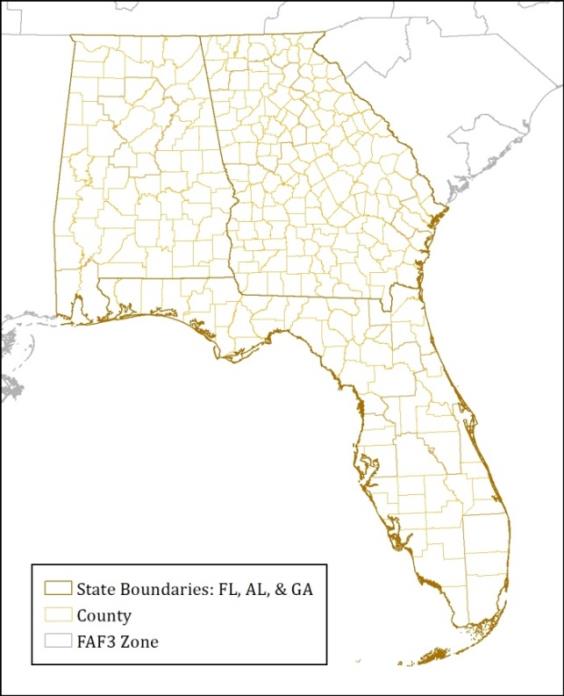
Figure 17. FAF Zones and Counties In Florida, Georgia, and Alabama.
Source: (RSG, 2015)

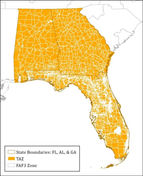
Figure 18. Statewide Traffic Zone System (Florida, Georgia, and Alabama).
Source: (RSG, 2015)

Data Inputs

Several data inputs were used for FreightSIM's development, both as main inputs or as additional, miscellaneous datasets. Table 4 lists a summary of the main inputs that are required for the model. This table lists each input and describes its source, the module(s) where it is applied, and an overview of the data.

Table 4. Data Sources for FreightSIM.

Type of Input	Input	Source	Description
Zone Systems	FAF3 Zone System	FHWA	Large regions, such as Combined Statistical Areas, or states
Zone Systems	County-Level Zone System	U.S. Census Bureau	Counties within FL/GA/AL
Zone Systems	TAZ-Level System	Florida Department of Transportation (FDOT)	TAZs within FL, counties (within the GA/AL) and FAF3 zones (outside of FL/GA/AL)
Network Elements	Network links	FDOT, Oak Ridge National Laboratory (ORNL) and U.S. Army Corps of Engineers	Highway (FDOT), rail (ORNL), and waterway network (U.S. Army Corps of Engineers) links
Network Elements	Transport and logistics nodes (TLN)	FDOT, ORNL, Bureau of Transportation Statistics (BTS)	Specific nodes within Florida; representative nodes outside of Florida
Network Elements	GCD	ORNL	Distance between all county-level O-D pairs in the United States
Network Elements	GCD to foreign zones	Created by project team	Distance between U.S. counties and foreign FAF3 zones
Economic Data	IO Make and Use Tables	U.S. BEA	Values of commodities exchanged between industries
Economic Data	Industry to Commodity Correspondence	FAME	List of SCTG commodities produced, by each NAICS6 industry
Economic Data	NAICS6 Industry to IO Industry Correspondence	U.S. BEA (2002)	Correspondences between detailed NAICS6 industries and aggregated NAICS IO industries
Freight Flows	FAF3 Commodity Flows	FHWA	Commodity flows between FAF3 zones
Freight Flows	Commodity Flow Survey	FHWA	Shipment sizes, by commodity and tonnages
Employment Data	CBP Data	U.S. Census (2010)	Employment, by industry
Employment Data	InfoGroup data	FDOT	Business operating in Florida
Validation Data	Truck Counts	FDOT	Medium and heavy truck counts
Validation Data	Truck Trip Origins and Destinations	American Transportation Research Institute	Sample of truck trips by county and TAZ O-D
Validation Data	Weigh-in-Motion (WIM) Data	FDOT	Truck weight distribution
Validation Data	Carload Waybill Data	U.S. Department of Transportation (USDOT) via FDOT	Complete restricted dataset of Carload Waybills
Validation Data	T-100 Data	BTS	Air freight segment and market data
Validation Data	Port Import/Export Reporting Service (PIERS) Data	FDOT	Import/export shipment data by port

Data Used for Estimating Model Parameters

FreightSIM uses the following main data sources for estimating model parameters:

• Supplier-Selection Model Parameters. Transferred from earlier freight modeling work for CMAP (Cambridge Systematics, 2011) and (Samimi A. M., 2010). Coefficients used as the probability of a supplier being paired with a buyer establishment (type). These coefficients were asserted and not estimated due to the unavailability of these data.
• Distribution Channel. Transferred from earlier modeling work for CMAP (RSG, University of Illinois at Chicago and John Bowman, 2012). The distribution channel model was estimated using data collected for a national survey as part of the FAME project (Samimi A. M., 2010).
• Shipment Size. Transferred from earlier modeling work for CMAP (RSG, University of Illinois at Chicago and John Bowman, 2012). The commercial vehicle surveys collected in Texas were used to estimate the model of shipment sizes.
• Mode and Transfer Choice. Mode and transfer choice model parameters were transferred from earlier freight modeling work for CMAP (Cambridge Systematics, 2011). This model was based on the formulation developed by de Jong and Ben-Akiva (de Jong, 2007). The formulation reflects the real-world decision-making of freight movers by accounting for different components of costs. Estimation of the parameters in the formulation was not possible without new data collection, but additional research on a few parameters led to revised assumptions for the Florida application:
  
  
  • Fixed cost per order (obtained from (Dominic, 2009) and (Benchmarks, 2006))
  • Storage costs per unit per year (based on the assumption provided in (Colonial Diversified, 2009))
  • Transportation and intermediate handling cost (adapted from (Leachman, 2005)).
  • Level-of-service parameters (adapted from (Leachman, 2005), (Bureau of Transportation Statistics, 2008) and (CSX, 2013)).
  • Path cost parameters (initial application in Chicago was a demonstration and these parameters were asserted (Cambridge Systematics, 2011) rather than estimated. Further research and consideration resulted in recommended values for several parameters).
  • Safety stock constants and categorization of commodities (based on the idea and assumptions in (Fisher, 1997)).
  • Lead time, standard deviation in demand and lead time and mode capacities (based on the research and assumptions in (Notteboom, 2011) and (CSX, 2013)). Lead time, standard deviation in demand, and lead time and mode capacities (based on the research and assumptions in (Notteboom, 2011) and (CSX, 2013)).
• Truck Payload and empty factors. Based on Vehicle Inventory and Use Survey (VIUS) data (VIUS, 2002).

Data Used for Model Calibration

FreightSIM uses the following main data sources for model calibration:

• Summaries of American Transportation Research Institute (ATRI) truck Global Positioning System (GPS) data (to support calibration of the distribution of truck trips).
• WIM data provided by FDOT (used during model calibration to inform adjustments to vehicle loading factors used to convert shipment tonnages to truck trips).
• The PIERS data provided by FDOT (used to develop calibration weights for the mode and transfers model, and the model of import and export volumes, by port).
• An online establishment survey done by University of Illinois at Chicago (Samimi A. M., 2010) results on proportions of shipments by distribution channel (used as calibration targets and for adjusting the alternative specific constants in the distribution channel model). The number of shipments by distribution channel type, commodity, and location were developed using the survey study results and were used to adjust the constants in the distribution channel model.
• CFS data on the distribution of shipment sizes by commodity (used as calibration targets and for adjusting the alternative specific constants in the shipment-size model).

Data Used for Model Validation

FreightSIM uses the following main data sources for model validation:

• TRANSEARCH commodity flows (used to validate mode and transfer choice model).
• Truck counts provided by FDOT (used to validate truck trip assignment model).

Table 5 shows the details of validation tests.

Table 5. FreightSIM Model Validation Tests.

Model Component	Validation Test	Data Source	Process
Shipments and their Size	Shipment size by establishment pair, commodity type	CFS TRANSEARCH data	Compare the shipment sizes and weights distribution by commodity
Mode-Transfer	Modal volume	TRANSEARCH data (incorporating Carload waybill data)	Compare mode shares by commodity group and movement/location
Truck Trip Assignment	Truck volumes	Highway truck counts, by vehicle type	Compare daily truck volumes by district, county, facility and screenline

Data Desired, but not Found

Some of the desired—but unobtainable—data for use in the model included the following:

• Data for estimating logistics costs calculations (e.g., storage costs, warehouse handling charge).
• Data for maximum load weight of truck types in the mode and transfer choice component of the model.

Detailed information about the model and the freight datasets is available online at:

• FreightSIM Wiki (enumerated web address: http://www.freightsim.net/).

WISCONSIN

Methodology

Supply Chain Modeling Needs

The Wisconsin Department of Transportation's (WisDOT's) main needs from its freight model are forecasts of truck volume on the roadways. WisDOT maintains data on the commodities being moved, and the origins and destinations of freight moving to, from, and through Wisconsin. WisDOT uses its freight model to answer the following questions:

• How many trucks are moved?
• Where are the trucks coming from and going to—locations within Wisconsin or outside of the State?
• What are the trucks carrying?
• How does truck volume or routing change based on the socioeconomic characteristics of an area or the freight facilities available?

WisDOT requires forecasts of trips by all modes that carry freight—not just trucks—to prepare these truck forecasts, evaluate changes in modal share, and provide forecasts of freight travel by other modes. Further, Wisconsin needs accurate tools and data for evaluating freight corridors entering Wisconsin, and for freight facilities in counties/metropolitan areas adjacent to Wisconsin.

WisDOT currently operates a vehicle trip-based model (where trips by different modes are not linked into supply chains). WisDOT has tested a supply chain model where the cargo carried by those trips are linked. According to WisDOT, the supply chain model as it was currently formulated, did not do a good job of evaluating changes in truck volume given changes in the socioeconomic characteristics of a given area, which was related to limitations inherent in the input data available. The inherent limitations of the input data are primarily related to the coarse granularity of the O-D freight flow data available to WisDOT (the FAF data). In one analysis scenario conducted as part of the model development, the model predicted fewer trucks going to and from Kenosha County—with the presence of a newly constructed Amazon fulfillment center there—than without it.

As tested by WisDOT, the supply chain model accurately predicts changes in mode shift due to changes in the use of supply chains or system inter-modality. In a different analysis scenario conducted as part of model development, the model showed that given the presence of an intermodal rail terminal in Milwaukee County, there would be an increase in mode share by rail containers in Wisconsin and nearby Minneapolis, Minnesota, and Rochelle and Chicago, Illinois. However, only a small portion of this freight tonnage was taken away from trucks, which are by far the dominant mode of freight transport in Wisconsin. (The supply chain model showed more rail tonnage taken away from the Minneapolis-area intermodal terminals than from the closer and more active Chicago terminals—this is counterintuitive to the expectations from adding a Milwaukee intermodal terminal.)

According to the agency, the short- and long-term applications of the WisDOT supply chain freight model are unclear at the time of writing this synthesis. The primary need of WisDOT from its freight model is to conduct evaluations like what was described in preceding paragraphs; WisDOT thinks that the supply chain model does not accurately evaluate truck volumes. There may be commodities or commodity groups where one model is preferable to another, particularly for mode allocation. For bulk commodities, the supply chain model seemed to slightly overestimate truck allocations, while also underestimating rail volumes. For finished goods, the supply chain model seemed to reverse this bias, with the rail mode seeing higher estimates than identified under the FAF. This appears to be a legacy of the origins of the modified Wisconsin supply chain model in the Chicago-area metropolitan planning organization's model; the presence of many intermodal facilities in the Chicago region allows greater opportunity for rail shipments of finished goods than in Wisconsin. Further, some freight movements are more conducive to a chain model, while others are better represented through O-D modeling. Examples of supply chain trips for Wisconsin's freight include the collection of milk by tanker trucks, the distribution of fuel oil or propane, and the wholesale or corporate distribution of consumer products at multiple retail locations.

Meanwhile, the O-D model best captures the movement of wood to paper mills, sand, and other aggregate to processing facilities, and coal to utility plants. Should the FAF be refined down to smaller regions, then that data could be used to test and compare the supply chain model with Wisconsin's existing trip-based model. Such a test could apply each model to a selection of typical bulk, semi-finished, and finished goods, evaluating the accuracy of that model against specific freight categories or commodities. The refined data would also better identify corridors and modes used for cross-border and multistate freight movements.

Model Structure, Component Interactions, and Segmentation

The Supply Chain Model includes the following component models:

• Firm synthesis.
• Supplier selection.
• FAF3 flow apportionment.
• Business location assignment.
• Distribution channel.
• Shipment size.
• Mode-path selection.

Figure 19 shows the Wisconsin freight model structure.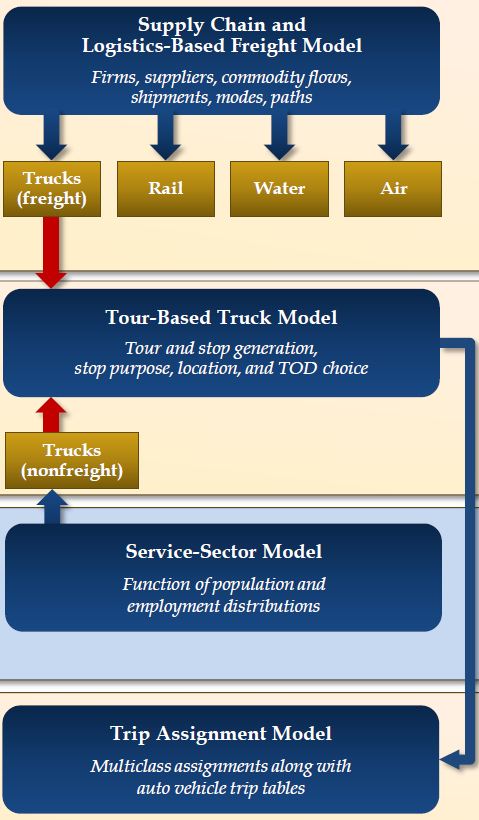

Figure 19. Wisconsin Freight Model Structure.
Source: (Cambridge Systematics, 2016)

The service sector model is not part of the supply chain model developed for WisDOT and it is included here for illustrative purposes only. A supply chain tour-based truck model was developed for WisDOT, but it did not yield meaningful information regarding local truck tours due to the coarse granularity of the underlying FAF3 input data. The lack of meaningful information was also attributable to the forecast usage of truck tours exclusively within supply chains (only truck tours occurring as part of supply chains were tested).

Market Segmentation (Industry, Commodity, Mode, Vehicle Type, Temporal, Activity Type)

Table 6 shows commodities and respective industries in the model. The model includes five modes (See Table 7).

Table 6. Wisconsin Model's Commodities and Industries.

Commodity	Industry
Live animals and fish	Farm products
Cereal grains (including seed)	Farm products
Other agricultural products, except for animal feed	Farm products
Animal feed and products of animal origin, n.e.c.	Food
Meat, fish, seafood, and their preparations	Food
Milled grain products and preparations, bakery products	Food
Other prepared foodstuffs and fats and oils	Food
Alcoholic beverages	Food
Tobacco products	Misc. nondurable manufacturing
Monumental or building stone	Nonmetallic minerals
Natural sands	Nonmetallic minerals
Gravel and crushed stone	Nonmetallic minerals
Nonmetallic minerals, not elsewhere classified	Nonmetallic minerals
Metallic ores and concentrates	Metallic ores
Coal	Coal and crude petroleum
Crude petroleum	Coal and crude petroleum
Gasoline and aviation turbine fuel	Petroleum products
Fuel oils	Petroleum products
Coal and petroleum products, not elsewhere classified	Petroleum products
Basic chemicals	Chemicals
Pharmaceutical products	Chemicals
Fertilizers	Chemicals
Chemical products and preparations, not elsewhere classified	Chemicals
Plastics and rubber	Rubber/plastics
Logs and other wood in the rough	Lumber
Wood products	Lumber
Pulp, newsprint, paper, and paperboard	Paper
Paper or paperboard articles	Paper
Printed products	Misc. nondurable manufacturing
Textiles, leather, and articles of textiles or leather	Misc. nondurable manufacturing
Nonmetallic mineral products	Clay, concrete, glass
Base metal in primary or semi-finished forms and in finished basic shapes	Metal
Articles of base metal	Fabricated metal products
Machinery	Machinery
Electronic and other electrical equipment and components and office equipment	Misc. durable manufacturing
Motorized and other vehicles (including parts)	Transportation equipment
Transportation equipment, not elsewhere classified	Transportation equipment
Precision instruments and apparatus	Misc. durable manufacturing
Furniture, mattresses and mattress supports, lamps, lighting fittings, etc.	Misc. nondurable manufacturing
Miscellaneous manufactured products	Misc. durable manufacturing
Waste and scrap	Waste
Mixed freight	Secondary traffic and drayage

Source: (Cambridge Systematics, 2016)

Table 7. Wisconsin Supply Chain Model's Mode and Vehicle Type.

Mode	Vehicle Type
Truck	Long-haul and local trucks
Rail	Vehicles not explicitly modeled or assigned—mode shares determined
Rail intermodal	Vehicles not explicitly modeled or assigned—mode shares determined
Water	Vehicles not explicitly modeled or assigned—mode shares determined
Air	Vehicles not explicitly modeled or assigned—mode shares determined

Source: (Cambridge Systematics, 2016)

The WisDOT's statewide supply chain freight model is an average daily model. Time-of-day assignment methods can be employed in tour-based truck models, but these were not employed in this test of the supply chain model for Wisconsin. The Wisconsin supply chain model forecasts multimodal cargo transport.

Modeled Performance Measures

The performance measures that are modeled in the WisDOT's statewide supply chain freight model are mostly the traditional performance measures:

• Tonnage, by mode (mode share).
• Truck volume.
• Truck volume-to-capacity. ²
• Truck VMT.
• Truck VHT.

Approach to Forecasting

The WisDOT statewide supply chain freight model as tested, was controlled by the basic multimodal O-D patterns in the FAF data. The model did forecast changes in the allocations of those multimodal O-Ds among different supply chains, but it was unable to change the multimodal O-D table in response to changes to Wisconsin's economy. By contrast, WisDOT's trip-based statewide model does forecast the multimodal O-Ds of freight based on changes in Wisconsin's economy.

Types of Applications and Procedures

WisDOT's statewide supply chain freight model was run on an R-Code platform and interface. It was not integrated with WisDOT's trip-based passenger model. Scenario creation typically involves making changes to network characteristics (like a proposed roadway capacity expansion or speed limit change) or socioeconomic characteristics (like proposed land development). All other model parameters are typically maintained between base and alternative scenarios.

Data

Geographic Scope

The WisDOT's statewide supply chain freight model zone structure is national for the allocation among supply chains, with greater detail within and near Wisconsin. The model zone structure for supply chain freight zones are counties in Wisconsin and neighboring states, the remainder of FAF regions in neighboring states, and FAF zones in all other U.S. States.

Data Inputs

• FAF commodity flow data.
• CBP data.
• TAZ shapefiles.
• Socioeconomic data (employment by type).
• IO Make and Use Tables (BEA).
• Highway and rail network shapefiles.
• Shapefiles of intermodal facility, distribution center, and warehouse locations.

Data Used for Estimating Model Parameters

The WisDOT model uses the following main data sources for estimating model parameters:

• FAF3 data (for payload factors).
• ATRI truck GPS data (for the truck-touring model parameters).
• VIUS data (for payload factors).
• University of Illinois's FAME model (for firm synthesis and supply chain allocation model parameters).

Data Used for Model Calibration/Validation

WisDOT performed a reasonableness check by aggregating the supply chain groups (e.g., direct truck, direct rail, air, water). Flows were also aggregated by commodity groups that were also used to renormalize the tonnages after the original allocation to supply chains. The results were then compared to the FAF modal and commodity group aggregations for calibration/validation. Since the allocation to supply chains were done to total tons over all modes, comparing with similar aggregations from FAF data means that the allocation worked correctly. The following main data sources were used for model calibration and validation:

• TRANSEARCH data.
• External station truck counts.
• Comparison of external flows vs. existing freight model flows.
• Comparison of freight mode shares vs. existing freight model shares.
• Truck VMT, by county.
• Vehicle classification data at specified screenlines.

Data Desired, but not Found

A county-level (or TAZ-level) multimodal freight cargo O-D table was the main data desired, but such an independent data source was not available for validation against the supply chain freight model's forecasts.

Detailed information about the model and the freight datasets is not yet available online.

PHOENIX

Methodology

The Maricopa Association of Governments (MAG), Arizona Department of Transportation (ADOT), and Pima Association of Governments (PAG) submitted a joint proposal to the SHRP2 C20 IAP to develop an operational megaregional multimodal agent-based behavioral freight model. The proposal was successful and in September of 2014 the work began. SHRP2 C20 IAP grant and additional support from the agencies provided necessary funding and in-kind contributions that allowed to successfully complete the project. The development took twenty-four months. As a result, a regional behavior-based freight transportation model was developed for the Arizona Sun Corridor megaregion for evaluating freight policy effects at the regional scale. Relevancy, importance, and timeliness of the model for the planning tasks was underlined by the fact that Arizona and the MAG region in particular rebounded from the recession. Arizona Sun Corridor megaregion, which includes MAG region, continues to be one of the fastest-growing megaregions in the country.

Supply Chain Modeling Needs

MAG, ADOT and PAG staff identified a need for the future development of the regional freight forecasting models. Arizona's Sun Corridor megaregion covers portions of five counties that include the MAG and PAG regions and is home to 8 out of 10 Arizonans. The Sun Corridor is also a major gateway for fresh produce and manufactured goods from busy freight ports on the U.S.-Mexico border. Arizona's population growth rate is expected to be robust in the upcoming decades and be one of the highest in the country, driven largely by activity in the Sun Corridor. FAF shows high growth rates in goods movement in Arizona. Given the expected growth in freight and its importance to the regional economy, MAG improved its capabilities to analyze freight demand in continuation of its state-of-the-practice truck models and developed a behavior-based freight modeling. MAG took a lead on the project and sought a behavioral-based freight modeling solution to support its organizational goals. MAG's goals included development of the regional transportation plan, development of freight transportation plans, and fostering transportation-related regional economic development. Moreover, MAG's extensive experience in developing and applying regional truck models led to a realization of the importance of behavior-based facets of freight decision-making. ADOT, MAG, and PAG realized that the decisions of shippers and carriers significantly affect regional transportation forecasting. A truck tour-based model recently developed by MAG resulted in noticeable improvements in forecast validations. The MAG's freight modeling tool addresses the changing conditions in freight supply and demand in the MAG region. It also captures transportation decisions, such as mode choice and the use of logistical handling facilities (e.g., intermodal yards) for individual establishments and simulates individual vehicle movements, allowing MAG to analyze impacts of new infrastructure projects at a highly detailed level.

Model Structure, Component Interactions, and Segmentation

The proposed modeling framework, that largely remained intact throughout the development, is shown in Figure 20. This figure provides information on the data inputs necessary to apply the individual modeling components in the new model system, data necessary to estimate various components of the supply chain and tour-based models, the supply chain models, key outputs that are produced from each modeling component, different geographic zones, and data that will be used to calibrate each component and validate the new model system. The flow chart detailing implementation of the supply chain, transport, mode, and path choice models is shown in Figure 21.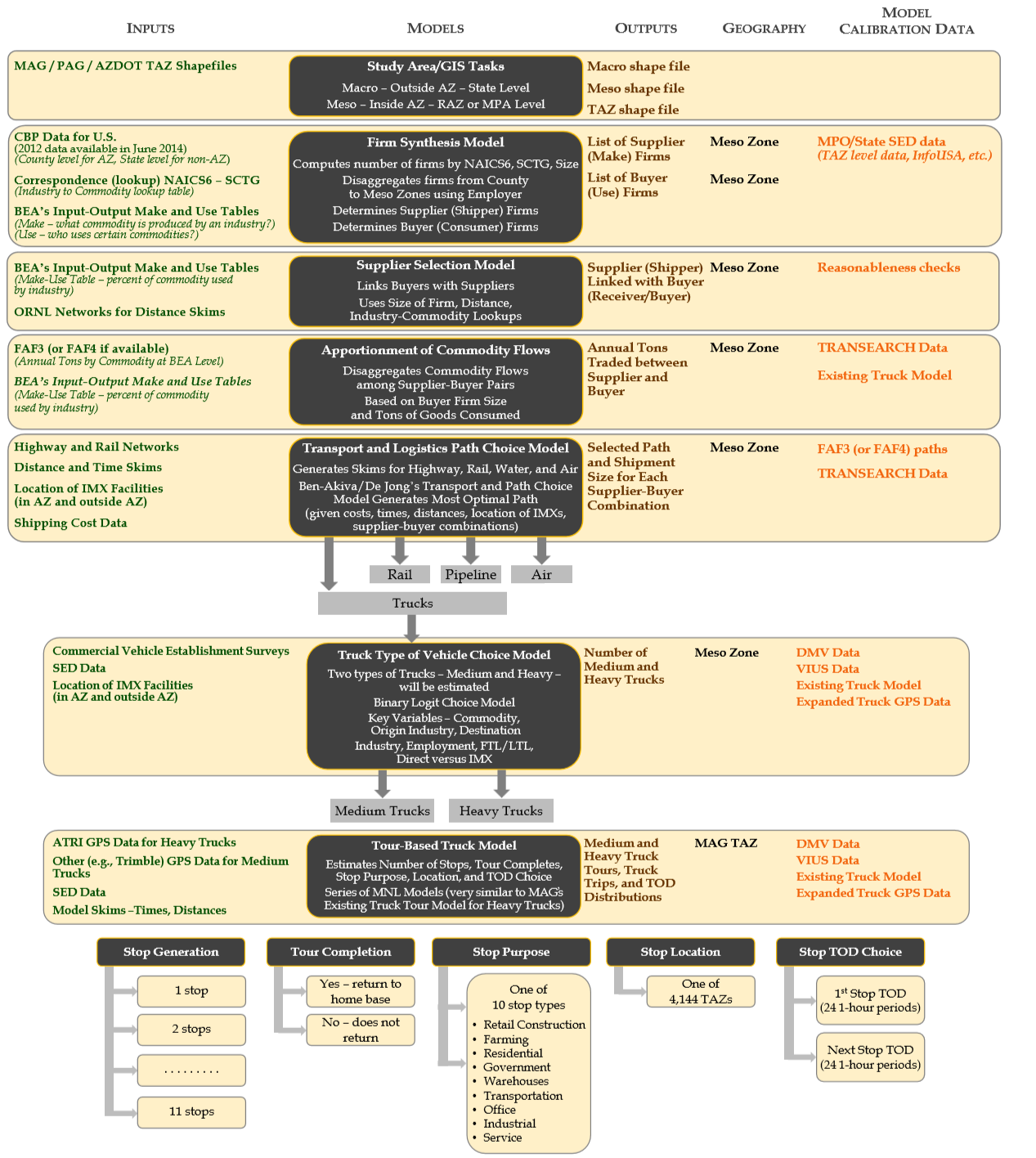

Figure 20. Individual Components Of The Proposed Behavior-Based Freight Model.
Source: (Maricopa Association of Governments, 2017)

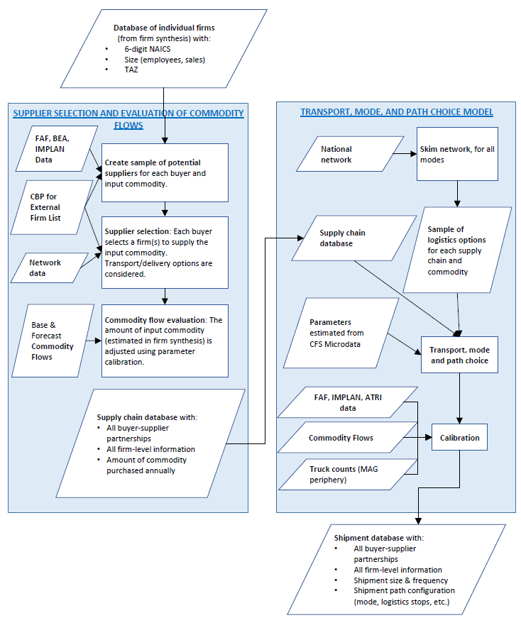
Figure 21. MAG Behavior-Based Supply Chain and Freight Transportation Framework.
Source: (Maricopa Association of Governments, 2017)

Overall freight modeling framework included the following three major components:

• Firm Synthesis Model. Synthesizes establishments and simulates regional establishments mainly by industry and by size in the base year and reflects firm evolution, including migration, creation, and dissolution of firms for future years. Georeferenced National Establishment Time-Series (NETS) data were purchased by MAG and used for the firm synthesis model development. The focus of the MAG firm synthesis model is on studying the three lifecycle events of the establishment beginning with birth, relocation, and death of the establishment in the study area. First, birth of an establishment is defined as the beginning (or first) year in which the business establishment was recorded in the NETS database for the MAG and PAG study area. Second, relocation is defined as change in address (or physical location) from one location to another. Finally, establishment death is defined as the last year in which the establishment and its internal attributes were recorded in the panel from 1990 to 2012. The model does not include businesses that were either formed or closed outside of the study area. Furthermore, business establishments were classified based on the two-digit NAICS codes to make the analysis tractable.
• Supply Chain and Supplier-Selection Model. Allocates commodities from producing establishments to those that need them. Establishments include those within the MAG/PAG megaregion and outside the region. The approach used in this model is an agent-based computation economics method that captures buyers' choices and suppliers' decisions relevant to buying and selling commodities. The model uses an algorithm that produces optimal and stable market allocations. The enumeration of establishments, calculation of production and consumption rates, and preparation of the supplier and buyer establishments data were developed in R. The supplier-selection algorithm was developed in Java.
• Transport, Mode, and Path Choice Model. Evaluates mode and shipment-size options jointly for each buyer-supplier partnership. A disaggregate joint model of mode choice and shipment size was estimated using the CFS 2012 Microdata sample as the primary source. Information on annual flows, including the origin, destination, and SCTG code of the shipment is obtained from the Supplier-Selection model. The path choice model evaluates options for breaking down the annual flows into individual shipments that are generated regularly throughout a typical year.
• Tour-Based Truck Model. Develops truck trip chains sorted by industry sector and by truck type. These truck trip chains are then grouped into the major linkages based on land uses the trucks make stops at and the probability of making another stop based on the number of previous stops. The tour-based model generates the number of stops by industry sector, number of stops on a tour, stop purposes, and the location and time of day of stops. Truck tours are modeled through a sequence of models, including predicting tour generation at the zonal level by tour purpose (i.e., starting land-use type), the number of stops for each tour, the purpose of those stops, the location of stops, and the time of day for stops. ATRI truck GPS data was used for the development of heavy truck tour models and a similar dataset for light and medium trucks was acquired from StreetLight.
• Vehicle-Type Choice Model. Employs a logit model using the data from the 2016 commercial establishment survey to predict the usage of heavy versus medium weight trucks by establishments in the MAG region. This survey collected data at 416 establishments in the MAG region.
• Assignment. Outputs annual commodity flows in tons by commodity group that require integration with the rest of the model system. From a highway assignment standpoint, only the truck flows from the supply chain model are used while rail, water, and other modes of freight are not assigned to any networks. The truck flows are converted to daily truck tours and trips and integrated with the highway assignment model.

Market Segmentation (Industry, Commodity, Mode, Vehicle Type, Temporal, Activity Type)

Forty-two classes of commodities based on the SCTG were considered in this model (with the exception of SCTG 42 - Miscellaneous Transported Products). Each class of commodity is considered as an independent economic market for which supply chains were determined. MAG staff developed Standard Transportation Commodity Code to SCTG crosswalk for two-digit codes to use the TRANSEARCH data for comparing the supply chain model output (including mode choice model) which were developed using the FAF data. The NAICS system is used for determining the industry class in the firm synthesis and supply chain models. Trip assignment of the truck trips was completed using the multi-class assignment technique for five vehicle types:

1. Single-occupant passenger vehicles.
2. High-occupant passenger vehicles with two or more occupants.
3. Light commercial trucks.
4. Medium trucks.
5. Heavy trucks.

Modeled Performance Measures

The performance measures that are modeled in the MAG freight model are mostly the traditional performance measures along with some indicators from the supply chain model:

• Tonnage by mode (mode share).
• Truck volume.
• Trip tables by truck type, time period, and user class.
• Truck VMT.
• Truck VHT.
• Establishments, by NAICS code.
• Producing tour statistics.
• Employment, by NAICS code.

Approach to Forecasting

The approach to forecasting and model development were based on a few main methodological principles:

1. Development of an agent-based model that will implement a micro-simulation approach to the freight system modeling in MAG region, including synthesis of establishments, disaggregation of relevant demo-economic data in the region, formation of supply-chain and establishment interaction models and tour-based travel models.
2. Development of a multi-modal freight model at least for major commodities relevant for the MAG-PAG mega-region based on commodity-based analysis of freight flows. High concentration of commodities and relatively limited number of large trip generators in the megaregion contribute to feasibility of this approach in order to capture main freight travel patterns. By providing an in-depth look at each segment of the industry it will be possible to better understand the drivers of each industry and model them specifically.
3. Behavioral approach to the model development, including modeling of the economic behaviors of establishments, shippers and carriers in generation of travel and tour formations. Examples of a freight agent's behavior can include the reaction of supply chains to variations in fuel price, global sourcing and manufacturing decisions and technology changes. The model can assist in coordinated policy development and can be an effective tool for improving freight operations.
4. Consideration of the MAG activity-based passenger modeling framework in order to facilitate future integration of the models. Model structure at this stage is envisioned including such major components as establishment synthesis, establishment interaction model, mode choice model and tour formation model.
5. Industry Specific – The model should be based in explanatory variables specific to each industry, which allows for industry related people to have a better understanding of the model and provide directly applicable data and feedback.

Types of Applications and Procedures

MAG uses its regional truck model for air quality conformity analysis, analysis of O-D patterns, bottlenecks, and infrastructure and land-use scenarios. MAG uses its freight model for forecasting. The newly developed megaregional freight model is tailored for more advanced analysis of economic policies and economic scenarios, including scenarios developed for areas that are outside of MAG's region but that affect its regional economy and freight flows. MAG planners (particularly the freight planning group) require freight model outputs. These outputs are also required by the MAG air quality division, MAG member agencies, and MAG member agency consultants. MAG also has commodity flow data—including TRANSEARCH data—at the TAZ level. MAG has used these data for future-year commodity flow forecasts, validation and calibration of freight models.

Data

Geographic Scope

The MAG freight model simulates freight shipments to, from, and within the Arizona Sun Corridor megaregion, which covers the Phoenix and Tucson Metropolitan areas in Maricopa, Pima, and Pinal counties. This region is home to more than 80% of the State's residents. Figure 22 shows the extent of the Sun Corridor megaregion.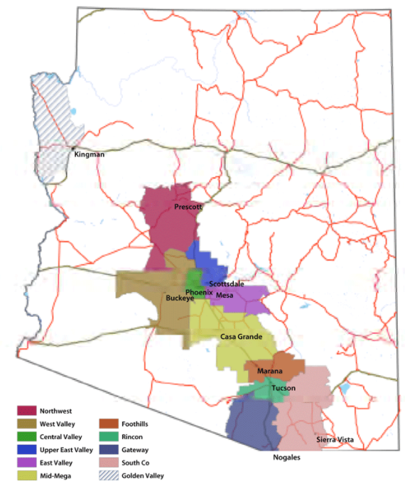

Figure 22. Sun Corridor Megaregion.
Source: (Maricopa Association of Governments, 2017)

The model focuses on regional commodity flows to/from/within MAG/PAG region. However, a variable zone system was used for the framework, which comprises finer zones in the Sun Corridor for more detailed analysis and larger zones for the external areas to Sun Corridor. The zone system includes TAZs in the MAG/PAG region, counties in the rest of Arizona, and FAF zones for the rest of the country. Figure 23 shows the zone system used in this model.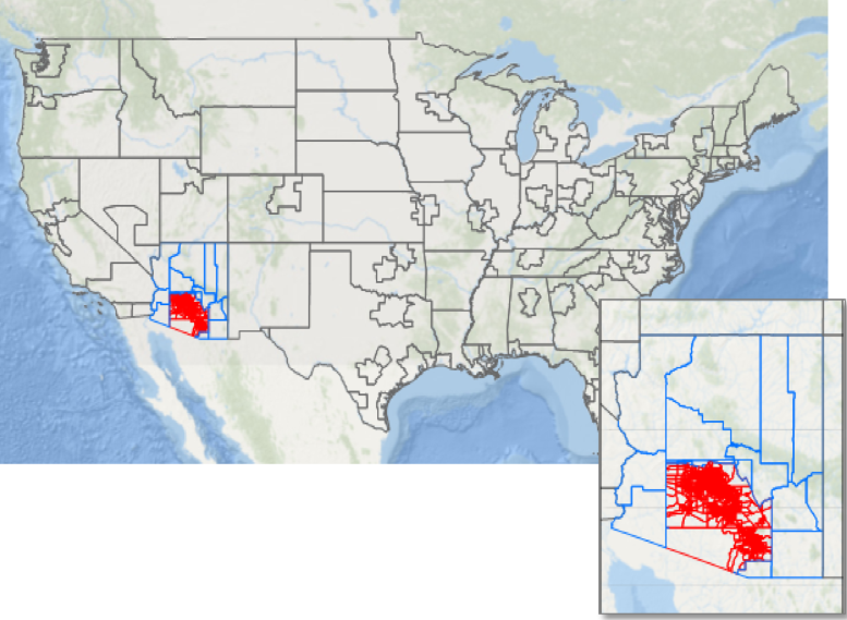

Figure 23. MAG Freight Model Zone System.
Source: (Maricopa Association of Governments, 2017)

Data Inputs

Firm Synthesis model utilized the following main datasets:

• NETS data.
• Employment data from CBP was used to generate establishments external to the Sun Corridor megaregion and to estimate industry-specific input and output factors. Firm synthesizer output was used to classify supplier and buyer agents in the megaregion area.
• MAG-PAG socio-economic data that includes regional population and employment.

The Supplier Selection Model used the following main datasets:

• Regional Make and Use Tables from Impact Analysis for Planning (IMPLAN )³. Regional Make and Use tables were used to calculate regional production and consumption rates by industry class per employee for all establishments in the megaregion.
• FAF4.1 data.
• IHS Global Insight's TRANSEARCH data.
• CFS 2012 Microdata for Arizona.
• MAG Regional Establishment Survey data.
• BEA IO Accounts tables, which contain Make and Use amounts of exchanged commodities between industries (at the six-digit NAICS level) were used to calculate amount of commodity produced and consumed on average per employee in each industry class for establishments outside the megaregion.
• National average and region—specific commodity prices derived from the FAF4.1 and Arizona-based sample of CFS PUM.
• A crosswalk was developed between FAF External Regions and MAG/PAG External stations to convert the foreign origin of a supply chain to MAG/PAG external station.
• Two Commodity-Industry Crosswalks that provide mapping between industries classes (six-digit NAICS and BEA IO industry classes) and the associated commodities (two-digit SCTG). These crosswalks were developed using the detailed description of SCTG and NAICS codes provided by U.S. Census Bureau and a preliminary commodity-industry bridge used in FAF data.
• BEA correspondence table that links BEA IO industry classes to NAICS six-digit industry classes.
• Aggregated inbound and outbound commodity flows at FAF-zone level derived from FAF4.1 data and used to calibrate estimated production and consumption amounts at establishment-level.
• GCD matrix calculated using the zoning system in the geographic information system (GIS) software.

The transport, mode, and path choice models were developed using the following main data sources:

• CFS 2012 microdata sample (the model development process used Arizona-based shipments).
• Multimodal transportation levels of service (developed by MAG): travel times, distances, logistics handling nodes (e.g., intermodal terminals and air cargo terminals), and number of rail tracks used (i.e., by track owner).
• Transportation costs for truck (less-than-truckload and truckload), rail, air, and parcel. This information is based primarily on BTS data and supplemented by rates found online.

The tour-based truck model development process used the following main data sources:

• ATRI truck GPS data. Maricopa Council of Governments (MAG) obtained samples from four different months.
• Streetlight data. Medium and Light Truck Tour models were developed using data from this vendor. MAG obtained data for April 2015.
• Land-use categories in Maricopa County, Pinal County and Pima County were different. MAG Truck model utilizes ten land uses. Hence, cross-walk tables were developed for each county, reconciling their land-use types with the ones referenced in MAG truck model, to facilitate Truck GPS data analysis.
• A crosswalk was developed between the Tour Type and Tour Purposes in Supply Chain and Truck Tour Models.
• Maricopa Council of –Pima Association of Governments socio-economic data that includes regional population and employment.
• VIUS uses product classes similar to the commodity classes used in the CFS or FAF or TRANSEARCH. The payload factors by each truck type and SCTG commodity were developed from the Arizona records in the 2002 VIUS database.
• Regional PM Peak skims.

Vehicle choice truck model development process used the following main data sources:

• 2016 MAG commercial establishment survey.

The process of developing independent networks for all main transportation modes that operate in Arizona used the following data sources:

• MAG modeling network.
• PAG modeling network.
• FAF3 roadway network.
• NTAD rail network.
• NTAD rail yards database.
• OpenFlights.org airport, airline, and route data (enumerated web address: https://openflights.org/data.html).
• U.S. BTS T100 segments database.
• MAG performed detailed analysis of the available freight data. The report on this research effort and detailed information about the datasets utilized for the model development are available from the MAG website.

Data Used for Estimating Model Parameters

MAG utilized NETS data from 1991 to 2011 for estimating establishment birth rates by industry type. CFS, Public Use Microdata (PUM) was used to estimate parameters in the transport, mode, and path choice model. ATRI and Streetlight data was used for estimating truck tour models. The unit value of commodities was asserted from FAF data. The supplier evaluation criteria were drawn from FAF (cost), synthesized firms (quality, reliability), network skims (delivery), and the GIS shapefile of zone system (distance). The transportation costs used in path choice model development were asserted from various sources like USDOT's Research and Innovative Technology Administration, among others.

Data Used for Model Calibration

The calibration of the model included calibration of the supplier-selection model and calibration of the mode choice model. FAF4.1 data was the main data source for calibration of both models. FAF4.1 commodity flow patterns to, from, and within MAG/PAG region were used for calibration of the supplier-selection model and the modal split in the FAF4.1 data was used for calibration of the mode choice model. The regional TRANSEARCH data sample was also considered and analyzed for the model calibration. However, it was not selected for the final calibration due to several inconsistencies that were found between TRANSEARCH and FAF data.

Data Used for Model Validation

The portion of NETS data that is left out of estimation is used to validate the model. This smaller set comprised 20% of the establishments that were randomly selected to avoid introducing bias into either set. Also, MAG desired a sufficient and comprehensive supplier-selection information (an establishment survey can gather that data) but it was not available. The survey questions should be focused on gathering information on the supplier-selection process, such as the scoring process by establishments of different sizes and industries. InfoGroup data and the Maricopa County Employer Database were also utilized in validating the output from Firm Synthesis model.

The assignment validation is done at two levels of geography. Screenlines analysis includes some of the major freeways that pass through the region and carry a large volume of trucks in the region.

Data Desired, but not Found

Data on the intermediate logistics nodes (e.g., consolidation centers, distribution centers) was desired but not available. The shipping chain choice could not be determined for truck shipments without these data. Instead, truck volumes were validated against observed count data. Lack of behavioral data on carriers, shippers, buyers, and suppliers effected the choice of the model methodologies.

Detailed information about the model and the freight datasets is available online at the following websites:

• Final Report for MAG Next Generation Freight Demand Model (enumerated web address: http://www.azmag.gov/Portals/0/Documents/TRANS_2017-02-13_SHRP2-C20-MAG-Next-Generation-Freight-Demand-Model-Update.pdf?ver=2017-04-06-112009-200).
• Review of Freight Data Sources for the Development of a Behavior-Based Freight Model (enumerated web address: http://www.azmag.gov/Portals/0/Documents/TRANS_2016-06-01_Review-of-Freight-Data-Sources-for-the-Development-of-a-BehaviorBased-Freight-Model.pdf?ver=2017-04-06-112000-513).

OREGON STATEWIDE

Methodology

Oregon's economy is growing faster than the national rate. Despite this growth, the Oregon Department of Transportation (ODOT) has only modestly increased the capacity of their State's highway system to meet growing demand over the last 20 years. Traffic congestion is rising quickly, affecting passenger travel and freight movement alike. Reliability is also declining while transportation infrastructure is aging, and revenue streams are shrinking. Oregon is an export-dependent State, relying heavily on the transportation system to get goods to market via highway, rail, water, and air. When transportation costs rise, Oregon's jobs and products are affected. Questions related to the trade-off associated with investing and disinvesting in the Oregon transportation system have been explored using the Oregon Statewide Integrated Model (SWIM). SWIM is one of the several tools and methods used to answer these questions. SWIM can also be used to estimate commodity flows, which is valuable to decision-makers and important to understanding regional economies and how they rely on the transportation system. ODOT has recently completed the development of the latest version of SWIM (version 2.5). Previous versions of the model (SWIM 1.0 and SWIM 2.0) are now retired and not being used by ODOT.

Supply Chain Modeling Needs

ODOT developed SWIM to evaluate the impact of actions related to transportation at the statewide level. Representing the fundamental economic forces influencing transportation and land-use activity was paramount in the model design. The supply chain modeling simulated how commodities are moved as freight by different modes of transport, such as marine, rail, and truck for a typical weekday. For trucks, shipments are simulated to appropriately transport daily commodity shipments modeled by the business activity allocation module of SWIM. ODOT has used this tool to evaluate the impacts of weight restricting bridges, recovering from a major earthquake, planning to meet the future demands on the system while facing aging infrastructure, and shrinking funding streams. SWIM has also been used to evaluate the uncertainty associated with economic growth and external shocks, such as rising fuel costs.

ODOT uses its integrated land-use transport economic model to answer the following policy, investment, and project assessments related questions:

• Where are the trucks coming from and going to—locations within Oregon or outside of the State?
• How does truck volume or routing change based on the socioeconomic characteristics of an area or the freight facilities available?

Model Structure, Component Interactions, and Segmentation

SWIM is an integrated economic land-use transport model covering the entire State of Oregon. SWIM system represents the behavior of the economy, land-use, and transport system in the State of Oregon and the interactions between them. The system is composed of a set of interconnected components that simulate different aspects of the full system. The structure of the overall model is shown in Figure 24. The following components are related to freight and commercial vehicle movements:

• The New Economics and Demographics (NED) component. Determines model-wide production activity levels, employment, and imports and exports based upon official Oregon State forecasts.
• The Activity Allocation (AA) component. Determines commodity (goods, services, floorspace, labor) quantity and price in all exchange zones to clear markets, including the location of business and households by beta zone.
• The Commercial Transport (CT) component. Generates mode split for goods movement flows and generates truck trips, combining shipments and possible trans-shipment locations, for a typical weekday. The CT module is written in the R statistical language.
• The External Transport (ET) component. Generates truck trips from through movements based on external station growth rates.
• The VISUM platform ⁴ . Assigns trips to a computer representation of the statewide transportation network, trips generated in the Person Travel (PT) Model and CT Model, generating routes with distance and travel time information.

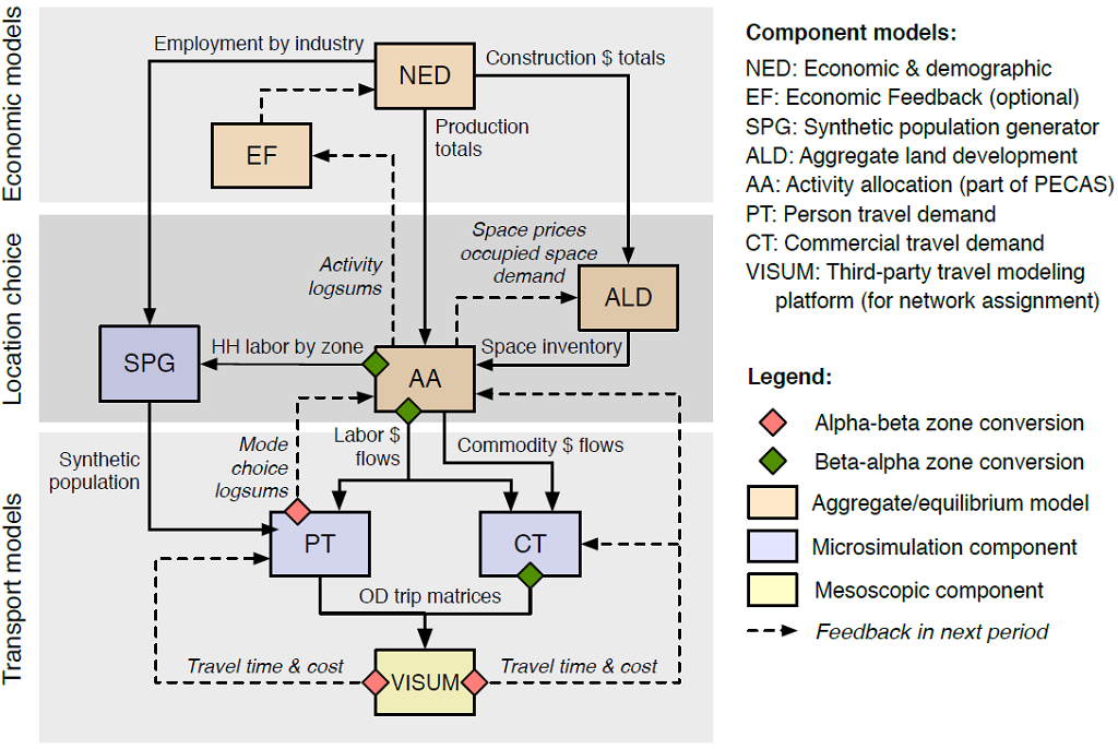
Figure 24. SWIM Overall Model Structure.
Source: (WSP, ECONorthwest, HBA Specto and RSG, 2017)

The model steps through time in one-year intervals, typically to a 20-year forecast horizon. The CT module is a hybrid framework that includes both aggregate and microsimulated data and models. The CT module includes several important dynamics unique to commercial vehicle travel:

• Represents explicit interaction with macroeconomic (NED) and AA modules.
• Represents supply chain linkages.
• Represents the complex structure of urban truck tours.
• Recognizes the large variances associated with freight activities.
• Integrates with the FHWA FAF.

Market Segmentation (Industry, Commodity, Mode, Vehicle Type, Temporal, Activity Type)

The commodities produced and consumed in the model, including model area imports and exports, are tracked in the AA and CT components, including 39 types of goods based on the SCTG categories. Some commodity groups are combined to eliminate small commodity flows and simplify the model. The various modes and vehicles used in the model to transport goods flows are shown in Table 8. Non-truck freight modes are not assigned to the network.

Table 8. SWIM Transport modes and vehicle types.

Code	Trip Mode	Definition	Component(s)
TRK1	Truck type 1	<34,000 lbs. (likely single-unit)	CT, ET
TRK2	Truck type 2	34,000–64,000 lbs.	CT, ET
TRK3	Truck type 3	64,000–80,000 lbs. (articulated)	CT, ET
TRK4	Truck type 4	80,000–105,500 lbs. (articulated)	CT, ET
TRK5	Truck type 5	>105,500 lbs. (articulated)	CT, ET
SAA	Air freight	Air freight (not assigned)	N/A
SRR	Rail freight	Rail freight (not assigned)	N/A
SWA	Waterborne freight	Waterborne freight (not assigned)	N/A

Source: (WSP, ECONorthwest, HBA Specto and RSG, 2017)

The industries defined in the NED and AA modules were built from data classified using different systems. IMPLAN data industries and NAICS code industries are used in these modules. Employment is forecast by IMPLAN sector (440 sectors) using a crosswalk and consistent with the official State economic forecast.

Modeled Performance Measures

ODOT does not use SWIM to generate performance measures, but metrics are developed to meet needs of specific analysis projects from SWIM. The metrics that are modeled and reported in SWIM and are used as part of the measures to analyze policy questions depends on the reliability of the input data that is accessible for each analysis project and on the purpose of the application. Some of the metrics that SWIM produces include:

• Average annual daily traffic.
• Regional share of Oregon Gross State Product.

Approach to Forecasting

The SWIM system runs on a dedicated multiprocessor personal computer. The modeling system is run using a Python script, which is called using a DOS command window to automatically set up the required directory structure. The script calls each component module, and runs the model through time. Each run of the model has its own base scenario directory structure that is a complete reference scenario run and stores full model outputs. The model steps through time in one-year intervals, typically to a 20-year forecast horizon. The NED model provides the starting point with the economic forecast information built from external data and forecasts from the State revenue forecast. The NED module provides model-wide production activity levels, employment, imports, and exports based upon the long-range forecasts consistent with the Department of Administrative Services' Oregon Economic & Revenue Forecast and the associated baseline macroeconomic forecast from IHS Markit. NED provides the starting point for the population synthesizer, AA module, land-use model, and PT and CT model to simulate people and business activity.

The CT module represents the flow of goods within the SWIM modeled area. It is designed to work closely with the AA module and complement the PT module. The current version of CT is written in the R statistical language, which is widely used at ODOT. Many of the models in the CT module are implemented as parallel processes using the doParallel package in R. The CT module reads the outputs produced by other modules and its own configuration and parameter files. Its output is a list of discrete truck trips and aggregate flows by commodity and mode. The CT program runs in 10–20 minutes, depending upon the number of cores and processor speeds.

Types of Applications and Procedures

SWIM has often been used to evaluate the economic effects of different investment scenarios. Modeling work completed to date includes evaluating the effects of weight-restricting bridges on heavy trucks, recovering from a major seismic event, impacts of higher vehicle operating costs and evaluating future investment options as infrastructure ages, construction costs rise, and funding streams shrink.

Data

Geographic Scope

SWIM operates at two geographic levels within the modeled area, which is shown in Figure 25. Both geographic levels encompass 36 counties within Oregon and 39 counties in adjacent states. The latter is commonly referred to as the model's halo area. The halo encompasses a roughly 50-mile buffer around Oregon comprising 39 counties in Washington, Idaho, Nevada, and California. A system of 2,950 alpha zones (light and dark lines in Figure 25) is the most disaggregate zone system. These include 12 external stations, shown in Figure 25. These external stations serve as gateways to the six world markets used to represent the world beyond the halo. The six world markets link to the model transport network at the 12 external stations.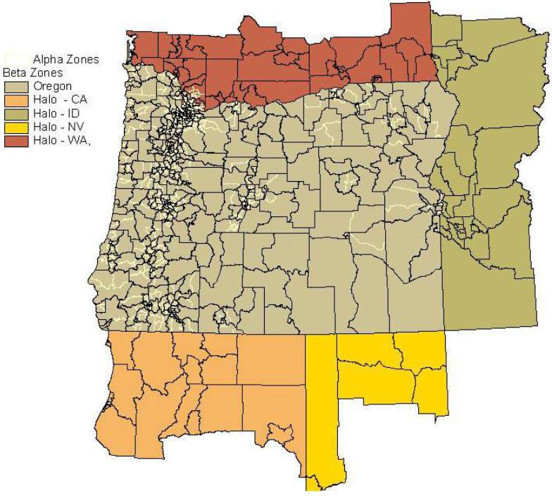

Figure 25. SWIM modeled area zone system.
Source: (WSP, ECONorthwest, HBA Specto and RSG, 2017)

SWIM represents the world outside of Oregon by FAF regions, which are aggregations of counties within the United States and countries or world regions outside of it. Within Oregon, the CT module operates at the alpha zone level. Because only Oregon and the halo are represented in the SWIM network, the interstate flows generated by CT module are routed through the external gateways.

Data Inputs

ODOT acquired and utilized the following datasets to develop the statewide supply chain freight model:

• CFS data (both publicly available and microdata).
• FAF data.
• IO Make and Use tables (BEA).
• VIUS data.
• Foreign trade statistics compiled by the U.S. Department of Commerce.
• Carload Waybill Sample (Surface Transportation Board).
• U.S. Army Corps of Engineers Waterborne Commerce data.
• BTS T100 segments air freight movement database.

The current version of CT relies heavily upon the FAF to depict long-distance freight flows.

Data Used for Estimating Model Parameters

SWIM used the following main data sources for estimating model parameters:

• CFS data.
• FAF data (to disaggregate FAF flows to smaller zones within a FAF region).
• VIUS data.

Data Used for Model Calibration/Validation

SWIM used the following main data sources for model calibration/validation:

• FAF4.
• ODOT traffic counts.
• Urban truck surveys from Denver, Houston, Ohio, Sydney, and Ontario.
• HERE data.⁵
• State and Portland CFSs.
• Information provided by stakeholders (this includes validation of truck routes patterns, industry employment locations, detour routes, and other local knowledge).

Data Desired, but not Found

Truck commodity flows by highway were the main data desired, but these data were unavailable.

Detailed information about the model and the freight datasets is available online at the following website:

• SWIM Version 2.5 Model Development Report (enumerated web address: http://www.oregon.gov/ODOT/Planning/Documents/Statewide-Integrated-Model-Vers2-5.pdf).

MARYLAND STATEWIDE/BALTIMORE REGION

Methodology

The Maryland State Highway Administration (SHA) and Baltimore Metropolitan Council (BMC) model is a two-agency freight model developed as part of the Freight and Commercial Vehicle Model Development project. The model work was completed in part with funding provided to SHA and BMC by FHWA under a SHRP2 C20 Implementation Assistance Program grant. The SHA/BMC model comprises two major components that function at different geographical scales. The larger, national-scale model that is designed for integration with the Maryland Statewide Model (MSTM) maintained by SHA is a supply chain model that simulates the transport of freight between supplier and buyer businesses in the United States, focusing on movements that include Maryland. As with the FreightSIM model of Florida on which it is based, the supply chain model produces a list of commodity shipments sorted by mode and converts those to daily truck trip tables that can be assigned to the national and statewide networks in MSTM along with trip tables from the passenger model component of MSTM. The second major component of the SHA/BMC freight model is a truck-touring model of the Baltimore modeling region, a 10-county area of Maryland. This regional portion of the model is a truck-touring model that simulates both freight trucks (using the supply chain model's shipment list as a demand input) and nonfreight commercial vehicles (using demand generated independently of the supply chain model).

Supply Chain Modeling Needs

SHA and BMC's application for the SHRP2 C20 grant outlined the planning needs that the SHA/BMC model is intended to support and was used to inform the development of the supply chain model. The agencies sought to develop modeling tools that provided some understanding of the connections between the region's economy, the resulting demand for freight movement, and the performance of the transportation systems. Three objectives informed the design of the model and supply chain modeling concepts:

• Agency needs for information on transportation system performance, with an emphasis on the role of freight movement and its role in the economic growth of the Baltimore region, Maryland, and the United States.
• The complexity of the regional transportation system—Maryland's position in the densely populated eastern seaboard and the congested Baltimore-Washington metropolitan region—increases the challenges of modeling freight movement.
• The desire to model long-distance truck movements, empty truck movements, local freight distribution, the effects of port expansions, and improvements to intermodal facilities.

The SHA/BMC model's design is a joint supply chain and truck-touring model where freight flows to and from the region influence vehicle movements at the local level to provide the desired modeling connections. For example, changes over time in the freight flows to and from a region influence the demand for long-distance truck travel and influence the need for additional local truck movements to facilitate local deliveries and pick-ups of shipments. The SHA/BMC model's geographical extent was designed to capture the full influence of the supply chains of shipments to and from the region. This model represents business establishments across the country and global suppliers and buyers who produce imports and consume exports. The model structure supports scenario testing to understand the effects of changes in the economy over time, including different patterns of long-haul domestic flows and imports and exports as domestic and international trading partners change.

Model Structure, Component Interactions, and Segmentation

The SHA/BMC model includes a national supply chain model (NSCM) and an urban truck-touring model, including the freight truck-touring model (FTTM) for freight and the commercial vehicle touring model (CVTM) for non-freight-carrying trucks. Figure 26 shows the overall model system used by SHA and BMC, which includes both the MSTM maintained by SHA and BMC's regional travel demand model. Both models contain passenger travel demand models that are used to estimate personal travel by auto and other modes. The components of the freight model are shared between the SHA and BMC models; the approach to integration between the two models is discussed below.

The NSCM comprises a firm synthesis model and a supply chain model. The NSCM simulates the transport of freight between supplier and buyer businesses in the United States and prioritizes movements that include Maryland. The model uses the output, a list of commodity shipments by mode, in two ways. First, in the MSTM, a model component connected to the NSCM converts the annual shipment flows to daily vehicle trip tables that can be assigned to the national and statewide networks in the MSTM along with trips tables from the passenger model. Second, the list of commodity shipments sorted by mode is used as an input to the FTTM in BMC's regional travel demand model.

The FTTM simulates truck movements within the Baltimore region that deliver and pick up freight shipments at business establishments. The FTTM is a tour-based model and builds a set of truck tours. These tours include transfer points at which the shipment is handled before delivery/after pick up for shipments with a more complex supply chain (i.e., a warehouse, distribution center, or consolidation center) and the suppliers and buyer of shipments where those are within the model region. The shipment list from the NSCM is used as the demand input for the FTTM and describes the magnitude and location of delivery and pick-up activity in the region that must be connected by truck movements. The model generates trip lists by truck type and time of day so that the outputs from this model can be combined with the outputs from the CVTM and appropriate passenger vehicle trip tables for highway assignment.

The CVTM simulates the remainder of the travel of light, medium, and heavy trucks for commercial service purposes (i.e., providing services and goods delivery to households and services to businesses). Like FTTM, the CVTM is a tour-based model, but demand is derived from the characteristics of the business establishments and households in the region and is not affected by the supply chain model. CVTM simulates truck and light-duty vehicle movements based on demand for services and goods from certain industries while FTTM simulates truck tours based on commodity flows.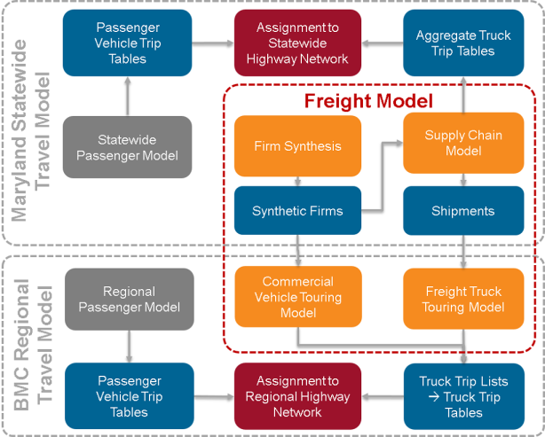

Figure 26. MSTM and BMC Model System.
Source: (RSG, University of Maryland, and Vision Engineering and Planning, 2017)

The NSCM includes components that synthesize business locations, trading relationships between businesses, and the resulting commodity flows, distribution channel, shipment size, and mode and path choice for each shipment made annually. A flow chart of the NSCM is shown in Figure 27. The transport and logistics chain models produce a list of shipments that are ready for extraction for use in the regional truck-touring model. This output is also converted into number of vehicles and loads ready for modal assignment (in this case, assignment is done for all truck trips to the highway network, to produce outputs of trucks volumes on the highway network, including to and from transfer facilities). The components shown in the flow chart perform the following model steps as part of firm synthesis and supply chain modeling:

Firm Synthesis

1. Business Establishment Synthesis. Synthesizes all business establishments in the United States and a sample of international business establishments using input employment data, which is more spatially detailed for the modeled region and less detailed for the rest of the United States; includes growth factors for future-year business synthesis.
2. Annual Production. Characterizes annual production by business establishments based on industrial classification.
3. Annual Consumption. Characterizes annual consumption by business establishments through relationships described in the IO data that describe the input commodities required to produce commodities.

Supply Chain Model

1. Buyer-Seller Matching. Selects supplier establishments for each buyer establishment by type, choosing one for each commodity input required by the buyer establishment.
2. Commodity Flow Allocation. Predicts the annual demand in tonnage for shipments of each commodity type between each establishment in the United States using input commodity flow forecasts.
3. Distribution Channels. Predicts the level of complexity of the supply chain (e.g., whether it is shipped directly or whether it passes through one or more warehouses, intermodal centers, distribution centers, or consolidation centers).
4. Shipment Size and Frequency. Estimates discrete shipments delivered from the supplier to the buyer.
5. Modes and Transfers. Predicts four primary modes (road, rail, air, and waterway) and transfer locations for shipments with complex supply chains using inputs from modal networks, including descriptions of transfer facilities.
6. Multimodal Network Flows. Produces a list of shipments for the transport and logistics chain model that are ready for extraction for use in the regional truck-touring model. This output is also converted into number of vehicles and loads ready for modal assignment (in this case, assignment is done for all truck trips to the highway network, to produce outputs of trucks volumes on the highway network, including to and from transfer facilities).

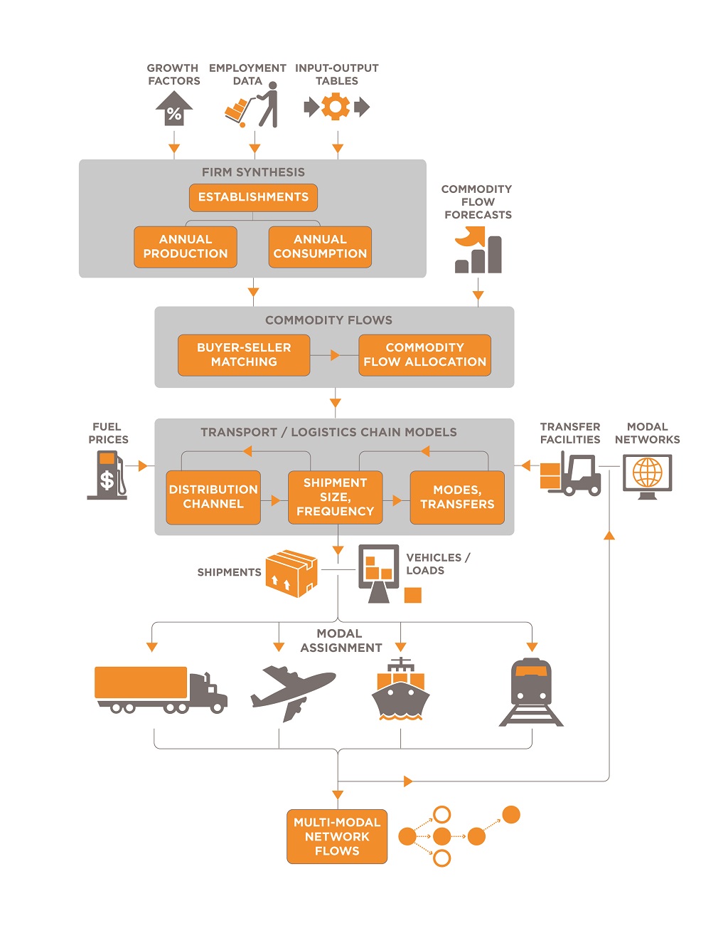
Figure 27. Components of the Supply Chain Model, SHA/BMC Model.
Source: (RSG, University of Maryland, and Vision Engineering and Planning, 2017)

Market Segmentation (Industry, Commodity, Mode, Vehicle Type, Temporal, Activity Type)

The SHA/BMC model system represents two major market segments for truck travel demand: freight movement and nonfreight commercial vehicle movement to provide services. The freight portion of the model—comprising the firm synthesis, supply chain model, and FTTM—contains several types of market segmentation depending on the unit of analysis of each model component.

The firm synthesis model characterizes business establishments by location (TAZ), establishment size (eight employment categories ranging from 1–19 employees to over 5,000 employees) and industry (six-digit Census Bureau NAICS categories). The number, type, and size of business establishments is controlled at the TAZ level within Maryland using the regional employment forecast data, which are grouped into seven employment categories that are aggregations of NAICS categories (i.e., retail, office, industrial, education, health services, food service, and other services). The commodity production and consumption by business establishment uses the BEA's six-digit NAICS categories (which is slightly aggregated in comparison to the U.S. Census Bureau's NAICS categories used for the industrial classification of the business establishments).

The supply chain model works with FAF commodity flow data and uses the 43 Standard Classification of Transported Goods categories for segmentation of shipment commodity. The distribution channel of the shipment flow through the supply chain is segmented into direct shipments, and those use one, two, or three transfers at distribution centers or intermodal transshipment locations. The supply chain model allocates shipments into size categories using a two-stage process, ultimately calibrating the distribution to the nine shipment-size categories, ranging from less than 50 pounds to more than 100,000 pounds used by the CFS. The shipments are allocated to one of four main modes (truck, rail, water, or air), with the intermodal paths being some combination of those modes (e.g., truck-rail-truck). The conversion to trip tables in the aggregate outputs from the supply chain model uses truck percentages for light, medium, and heavy trucks (FHWA class 2–3, 4–7, and 8–13, respectively). The trip tables are divided into four time-period-specific trip tables (AM peak, midday off-peak, PM peak, and nighttime off-peak) using fixed factors.

The truck-touring model in the SHA/BMC model uses the same vehicle-type categories (light, medium, and heavy trucks) as the supply chain model's aggregate trip table outputs. The output trip roster from the truck-touring model has trip start and end times defined by minute of the day. These can be aggregated as needed into time period trip tables for static assignment. The stops that trucks make in the region are segmented into a series of different activity types. Scheduled stop activities (i.e., those where the truck is conducting its primary business) include delivery of a shipment, pick-up of a shipment, service activity, and meeting (with the latter two only relevant for nonfreight commercial vehicles). The model also adds intermediate stops for meals/breaks, vehicle service/refueling, and other purposes.

Modeled Performance Measures

The outputs from the SHA/BMC freight model include databases of business establishments, shipments by mode, and truck trips. The truck trips are aggregated into zone-to-zone trips tables and assigned to both the statewide and regional highway networks to give medium and heavy truck class volumes, by link.

The SHA/BMC freight model can produce the following performance measures from the model outputs:

• Annual tonnage shipped by mode to, from, and within Maryland, by SCTG commodity. These results are available at the TAZ level using both the statewide and regional zones (the latter is for the BMC model region).
• Mode shares of shipments by commodity and origin/destination, including imports and exports.
• Truck origin/destination patterns by truck type, activity, and time of day.
• Truck volumes by truck type, time period, and link on both the Maryland Statewide Model and BMC highway networks, which can be used to derive measures such as VMT and vehicle hours traveled (VHT) aggregated spatially by area type, functional class, and facility.

Approach to Forecasting

The SHA/BMC freight model is integrated into both the Maryland Statewide Transportation Model (MSTM) and BMC's regional travel demand model. MSTM and the BMC's regional travel demand model are loosely integrated. SHA has assumed responsibility for the NSCM integrated within their MSTM and BMC has assumed responsibility for the FTTM and CVTM models integrated within their regional travel demand model. In this loose integration, the two parts of the model will operate independently. However, the outputs from the synthetic establishments located in the BMC region and the shipments traveling into, out of, and within the BMC region will be created by the NSCM within the MSTM. These outputs will then be provided as inputs to the urban freight modeling system (FTTM and CVTM) within the BMC regional travel demand model. For forecasting future scenarios, the firm synthesis model adjusts to match the input employment data at the TAZ level.

The two agencies cooperate on employment forecasts and now use a consistent seven-category employment system, so the output business establishment database is appropriately adjusted for use in future years at both the statewide and regional level. The supply chain model's main future-year and alternative scenario inputs are commodity flow data and network inputs. By default, FAF forecasts are included as commodity flow data inputs, but the model user can adjust inputs to evaluate scenarios with alternative future commodity flows. The network inputs include forecasted changes in daily travel times and distances due to network changes (to highway, rail networks, and waterways) and to intermodal/transfer locations (e.g., rail yards, ports, airports, and truck terminals/distribution centers). The truck-touring models use the more detailed time-period-specific skims as the truck-touring models are sensitive to congested travel times by time period. As a result, forecasting in these models requires future-year scenario networks and the requirement of producing forecasted passenger trips to support joint assignment of passenger trips and truck trips.

Types of Applications and Procedures

The SHA/BMC freight model supports policy decision-making objectives, including project planning, corridor studies, and freight tolling. At the regional level, BMC staff use model simulation to support long-range plan development and federal transportation conformity determination. BMC staff use model outputs in regional transportation system performance measures of mobility, accessibility, equity, and environmental effects presented to committees. At the corridor level, performance measures of link level of service, travel speeds, and cost will be used at the project-planning level. These performance measures should be sensitive to existing and emerging transportation planning scenarios such as additional travel lanes, new interchanges, truck prohibitions, managed/electronic toll lanes, and freight generation scenarios such as port expansion or new intermodal transfer facilities.

Data

Geographic Scope

The supply chain model, which is integrated with the MSTM, has a global geographic scope. At its broadest, it represents import and export movements to and from eight international zones. Domestic movements are represented to and from the rest of the Unites States, and the model design includes simplified transportation networks that cover the entire continental United States. The model uses the MSTM TAZ, system, which is more spatially detailed in portions of the states surrounding Maryland, and then more highly detailed within the State of Maryland. Figure 28 shows the North American extent of the model's zone system, and Figure 29 shows the State of Maryland and the halo of smaller zones around the State. The national transportation networks are connected to detailed transportation networks covering Maryland. The regional freight and CVTMs cover the BMC modeling region. Figure 30 shows the BMC modeling region and the TAZ boundaries within the region.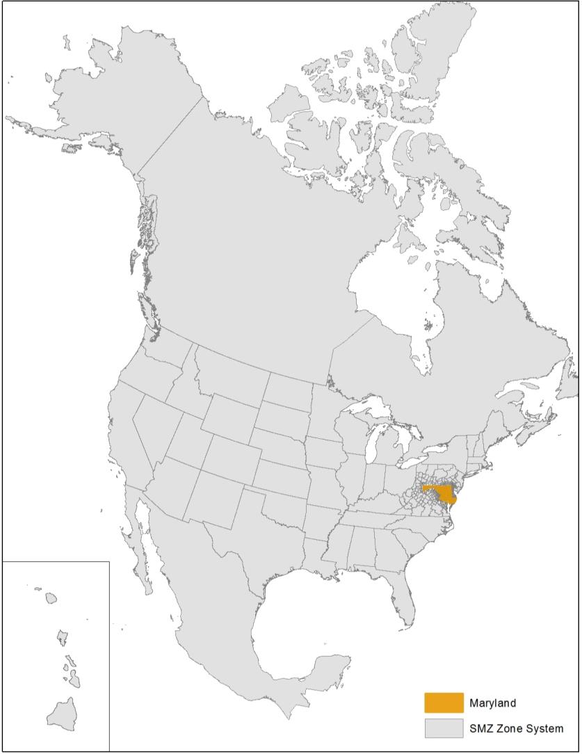

Figure 28. SHA/BMC Model Zone System, North American Extent of MSTM Zones.
Source: (RSG, University of Maryland, and Vision Engineering and Planning, 2017)

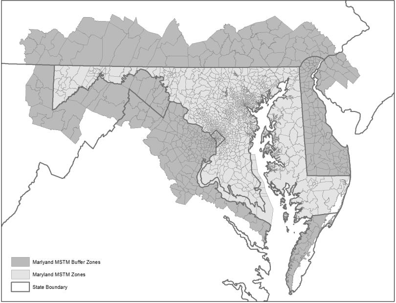
Figure 29. SHA/BMC Model Zone System, Maryland, and HALO Extent of MSTM Zones.
Source: (RSG, University of Maryland, and Vision Engineering and Planning, 2017)

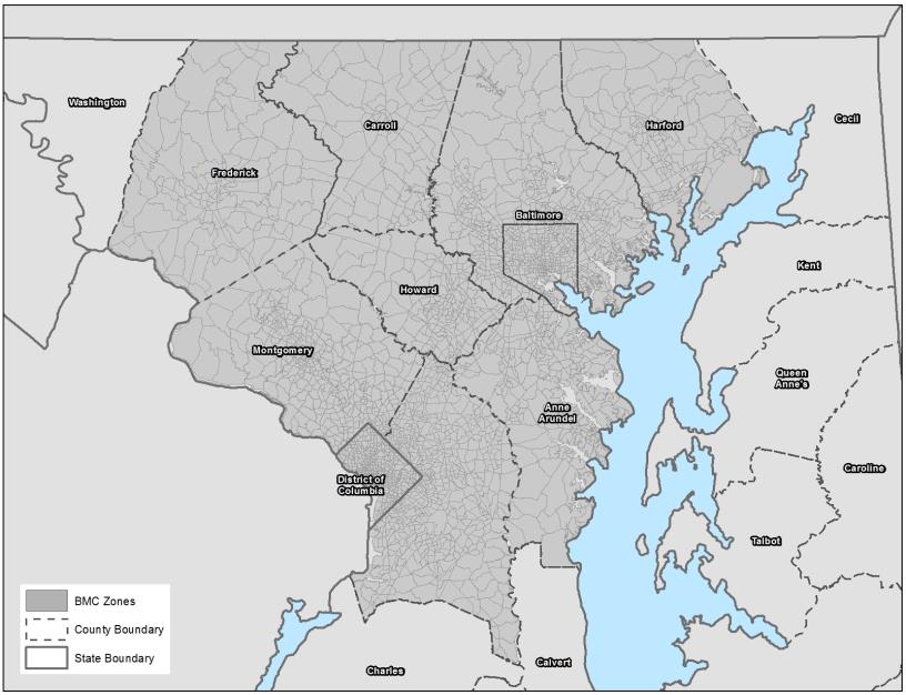
Figure 30. SHA/BMC Model Zone System, Extent of BMC Regional Zones.
Source: (RSG, University of Maryland, and Vision Engineering and Planning, 2017)

Data Inputs

The SHA/BMC models use the following main data sources as input:

• Zone Systems. MSTM zone system developed by SHA; combination of U.S. states and TAZs around and within Maryland; BMC regional travel model zone system developed by BMC; and county-level zone system (U.S. Census Bureau).
• Economic Data. IO Make and Use tables (BEA) and industry to commodity correspondences (BEA and FAME).
• Employment Data. CBP data (U.S. Census Bureau) and SHA and BMC employment data sorted by TAZ. LEHD data by Census block for allocation from counties to smaller geographical units.
• Commodity Flow Data. Commodity Flow Data from the FAF4 (FHWA).
• Networks. SHA's MSTM national highway network and BMC's regional travel demand model network used for highway skims and assignment. The model's nonfreight networks for rail, waterways, and the locations of ports, airports, and intermodal facilities are based on the National Transportation Atlas Database (NTAD).
• Distribution Centers and Warehouses. Database of the locations of distribution centers and warehouses developed from employment data with visual confirmation using Google maps.

Data Used for Estimating Model Parameters

The SHA/BMC model used the following main data source for estimating model parameters:

• Data collected for a national survey as part of the FAME project (Samimi A. M., 2010). Estimates the distribution channel model transferred from the earlier CMAP model.
• Commercial vehicle surveys collected in Texas. Estimates shipment sizes and several of the components of the FTTM, which were transferred from the earlier CMAP model described above.
• Research conducted by de Jong and Ben-Akiva (de Jong, 2007). Adapts research to use in the mode and intermediate transfer model to predict the mode and path of long-haul movements of freight based on a comprehensive accounting of transport and logistics costs.
• Ohio General Establishment Survey (Ohio DOT). Estimates several of the components of the CVTM and FTTM using establishment and truck diary survey.

Data Used for Model Calibration and Validation

The SHA/BMC model calibration and validation process relied on the following sources:

• Shipment-size distributions from the 2012 CFS.
• Proportions of shipments using direct or complex distribution channels based on the FAME survey.
• Mode choices by commodity and trip type segment (e.g., internal to internal, internal to external) from FAF4.
• Payloads and empty truck proportions from the 2002 VIUS.
• Distributions from the Ohio General Establishment Survey.
• ATRI truck GPS sample (distributions and O-D data derived by expansion using counts).
• Classified truck counts.

Data Desired, but not Found

Some of the desired—but unobtainable—data for use in the model included the following:

• Local data on shipping and truck travel behavior (e.g., collected using a regional establishment survey).
• Truck GPS data focused on light and medium commercial vehicles.
• Detailed data on commodities handled at individual distribution centers, warehouses, and intermodal facilities.

Detailed information about the model and the freight datasets is not yet available online.

PORTLAND METRO

Methodology

Metro received a SHRP2 C20 grant and is currently developing a new behavior-based freight and commercial vehicle modeling system. The current model development effort will produce three major components:

• NSCM. Connects the Portland region with the rest of the nation and includes global freight flows based on FAF data.
• Tour-Based Freight Truck Model. Encompasses freight delivery and pick-up movements, which converts shipments generated by the supply chain model into local truck trips.
• Tour-Based Nonfreight Commercial Service Model. Generates trips based on local land uses for both commercial and residential customers.

Supply Chain Modeling Needs

The new freight model will replace Metro's current trip-based truck model that utilizes fixed commodity flows with a joint supply chain freight model and truck-touring model designed to reflect decisions made by shippers, receivers, truck operators, terminal managers, and others. The model simulates movement of individual shipments throughout the supply chain, including both direct shipments, and those that traverse transshipment facilities. The model simulates movements of all freight shipments over one year and then simulates a representative sample of shipments on an average weekday in the truck-touring model.

The objectives of the model and the project are as follows:

• Develop tools to enable a more comprehensive analysis of infrastructure needs and policy choices pertaining to goods movement.
• Develop more detailed network assignments by truck type to support regional environmental analysis, and local traffic operations and engineering analysis.
• Develop freight forecasts that are responsive to changes in economic forecasts, changing growth rates among industrial sectors, and changing rates of economic exchange and commodity flows between sectors.
• Replace trip-based truck model with advanced tour-based model.

These objectives are identified by key participants in the project including Metro, Oregon Department of Transportation, the Ports of Portland and Vancouver, the Portland Freight Committee and several local agencies (e.g., City of Portland, Southwest Regional Transportation Commission, and Clackamas County).

In applying for the grant to develop the model, Metro recognized the need for coordinated freight planning and freight's role as an economic engine for the region. This recognition facilitated the collection of freight data and the development of a new freight model. The freight model is being developed using the framework developed for FHWA and previously implemented as a demonstration project for CMAP. The model specification is being customized for the Portland metropolitan region and model parameters are being estimated or calibrated using data collected in a locally funded survey and passive data collection effort. The model uses simulated commodity flows between industrial sectors to estimate external flows into and out of the region for local producer and consumer entities, consistent with State and regional economic forecasts.

Model Structure, Component Interactions, and Segmentation

The Metro freight model is based on a combined supply chain and tour-based framework developed with FHWA research funding and implemented in Chicago and Florida with RSG's rFreight" software. This framework comprises several steps that simulate the transport of freight between each supplier and buyer business in the United States. Figure 31 shows the supply chain processes and identifies major input and output data.

Figure 31. Metro Supply Chain Model Structure.
Source: (DKS, RSG, and Synergy Associates, 2017)

The modeling system sequence includes selection of business locations, trading relationships between businesses, and the resulting commodity flows, distribution channel, shipment size, and mode and path choices for each shipment made annually:

• Firm Synthesis. Synthesizes all establishments in the United States and a sample of international establishments.
• Supplier Firm Selection. Selects supplier establishments for each buyer establishment, by type.
• Goods Demand. Forecasts the annual demand in tonnage for shipments of each commodity type between each establishment in the United States.
• Firm Allocation. Allocates establishments in each county to TAZs within the Portland region.
• Distribution Channels. Predicts the level of complexity of the supply chain (e.g., whether it is shipped directly or whether it passes through one or more warehouses, intermodal centers, distribution centers, or consolidation centers).
• Shipment Size and Frequency. Estimates discrete shipments delivered from the supplier to the buyer.
• Modes and Transfers. Predicts four primary modes (road, rail, air, and waterway) and transfer locations for shipments with complex supply chains.

The supply chain model integrates with a regional truck-touring model, which is a sequence of models that takes shipments from their final transfer point to their final delivery point. The integrated modeling system connects the NSCMs with the regional truck-touring models. The final transfer point is the last point at which the shipment is handled before delivery (i.e., a warehouse, distribution center, or consolidation center for shipments with a more complex supply chain or the supplier for a direct shipment). It performs the same function in reverse for shipments at the pick-up end, where shipments are taken from the supplier to distances as far as the first transfer point. For shipments that include transfers, the tour-based truck model accounts for the arrangement of delivery and pick-up activity of shipments into truck tours.

The Metro model also includes a separate CVTM to simulate the remaining nonfreight truck movements in the model region that are not captured by the FTTM. The two truck-touring models have been transferred from the new SHA/BMC freight model described in this synthesis and have been either estimated or calibrated using the local data collected during the Portland model project.

The Metro freight model will be integrated with the passenger travel model and be part of the Metro travel demand modeling system. While the NSCM is not sensitive to local congested travel times within the Portland region—it is run using travel times and costs skimmed from a separate multimodal network—the two truck-touring models will be included within the Metro's travel demand model's feedback loops and use congested travel time skims as inputs. This means that the truck-touring patterns are sensitive to local congestion.

Market Segmentation (Industry, Commodity, Mode, Vehicle Type, Temporal, Activity Type)

The Metro freight model represents two major market segments in terms of demand for truck travel: freight movement and nonfreight commercial vehicle movement to provide services. The freight portion of the model—comprising firm synthesis, supply chain model, and FTTM—contains several different types of market segmentation depending on the unit of analysis of each model component.

The firm synthesis model characterizes business establishments by location (TAZ), establishment size (eight employment categories ranging from 1–19 employees to over 5,000 employees) and industry (six-digit Census Bureau NAICS categories) and is controlled at the TAZ level within the Metro region using regional employment forecast data. This is grouped into 14 employment categories that are aggregations of NAICS categories. The commodity production and consumption by business establishment uses the BEA's six-digit NAICS categories, which is slightly aggregated in comparison to the U.S. Census Bureau's NAICS categories used for the industrial classification of the business establishments.

The supply chain model works with FAF commodity flow data and uses the 43 SCTG categories for segmentation of shipment commodity. The distribution channel of the shipment flow through the supply chain is segmented into direct shipments using one, two, or three transfers at distribution centers or intermodal transshipment locations. The supply chain model allocates shipments into size categories using a two-stage process, ultimately calibrating the distribution to the nine shipment-size categories, ranging from less than 50 pounds to more than 100,000 pounds used by the CFS. The shipments are allocated to one of four main modes (truck, rail, water, or air), with the intermodal paths being some combination of those modes (e.g., truck-rail-truck).

The truck-touring model uses light, medium, and heavy trucks (FHWA classes 2–3, 4–7, and 8–13, respectively) for vehicle-type categories. The output trip roster from the truck-touring model has trip start and end times defined by minute of the day. These can be aggregated into time period trip tables for static assignment. The stops that trucks make in the region are segmented into a series of different activity types. Scheduled stop activities (i.e., those where the truck is conducting its primary business) include delivery of a shipment, pick-up of a shipment, service activity, and meeting (with the latter two only relevant for nonfreight commercial vehicles). The model also adds intermediate stops for meals/breaks, vehicle service/refueling, and other purposes.

Modeled Performance Measures

The outputs from the Metro freight model include databases of business establishments, shipments by mode, and truck trips. The model aggregates truck trips into zone-to-zone trips tables and assigns these to the regional highway network to produce medium and heavy truck class volumes sorted by link. The following performance measures can be derived from the model outputs:

• Annual tonnage shipped by mode to, from, and within the Metro region by SCTG commodity. These results are available at the TAZ level.
• Mode shares of shipments by commodity and origin/destination, including imports and exports.
• Truck origin/destination patterns sorted by truck type, activity, and time of day.
• Truck volumes by truck type, time period, and link on the Metro highway network, which can be used to derive measures such as VMT and VHT aggregated spatially by area type, functional class, and facility.
• During scenario testing model users can select commodities or groups of commodities to trace through the model, including assigning to the highway network as a separate class.

Approach to Forecasting

The Metro freight model is being integrated into Metro's regional travel demand model. For forecasting future scenarios, the firm synthesis model adjusts to match the input employment data at the TAZ level. The supply chain model's main future-year and alternative scenario inputs are commodity flow data and network inputs. By default, FAF forecasts are included as commodity flow data inputs, but the model user can adjust these to evaluate scenarios with alternative future commodity flows. The network inputs include forecasted changes in daily travel times and distances due to network changes (to highway, rail networks, and waterways) and to intermodal/transfer locations (such as rail yards, ports, airports, and truck terminals/distribution centers). The truck-touring models use the more detailed time-period-specific skims because the truck-touring models are sensitive to congested travel times by time period. Thus, forecasting in these models requires future-year scenario networks for the Metro region and forecasted passenger trips to support joint assignment of passenger trips and truck trips.

Types of Applications and Procedures

The Metro freight model is multimodal and can evaluate the effect of infrastructure projects on system performance:

• Highway Capacity Projects. Adding general purpose lanes.
• Managed Lane Projects. Adding truck-only lanes or managed lanes prohibiting trucks.
• Rail Capacity Projects. Adding service or new terminals/routes and improving access/egress to rail terminals.
• Port Capacity Projects. Adding terminals and improving access/egress to ports.
• Transfer Facility Projects. Adding intermodal terminals or distribution centers and improving access/egress to terminals or centers.

The Metro freight model can support the following types of transportation planning projects:

• Regional transportation plans with a freight component.
• Tolls, user fees, or pricing studies, such as traffic and revenue and congestion pricing studies.
• Corridor studies and alternative analysis.
• Land-use and environmental impact studies.
• Congestion management studies.
• Accessibility to manufacturing and industrial centers.
• Operational studies, effect on speeds, and travel times.

The Metro freight model can also help evaluate the effects of private sector decisions, such as just-in-time delivery, night deliveries, and adding or moving warehouse and distribution centers.

Data

Geographic Scope

The Metro supply chain model has a global geographic scope. At its broadest, it represents import and export movements to and from international FAF zones. For the Metro model, given the proximity to Canada, the single Canadian FAF zone has been disaggregated into multiple zones based on groupings of provinces. Domestic movements are represented to and from the rest of the United States, and the model design includes simplified transportation networks that cover the entire continental United States. The model uses the FAF TAZ system and includes additional spatial detailed in Oregon and Idaho. The freight model uses the same TAZs as the current regional travel demand model within the four-county Metro region. Figure 32 shows the North American extent of the model's zone system, while Figure 33 highlights Oregon and Idaho. The regional freight and CVTMs cover the Metro modeling region. Figure 34 shows the Metro modeling region and the TAZ boundaries within the region.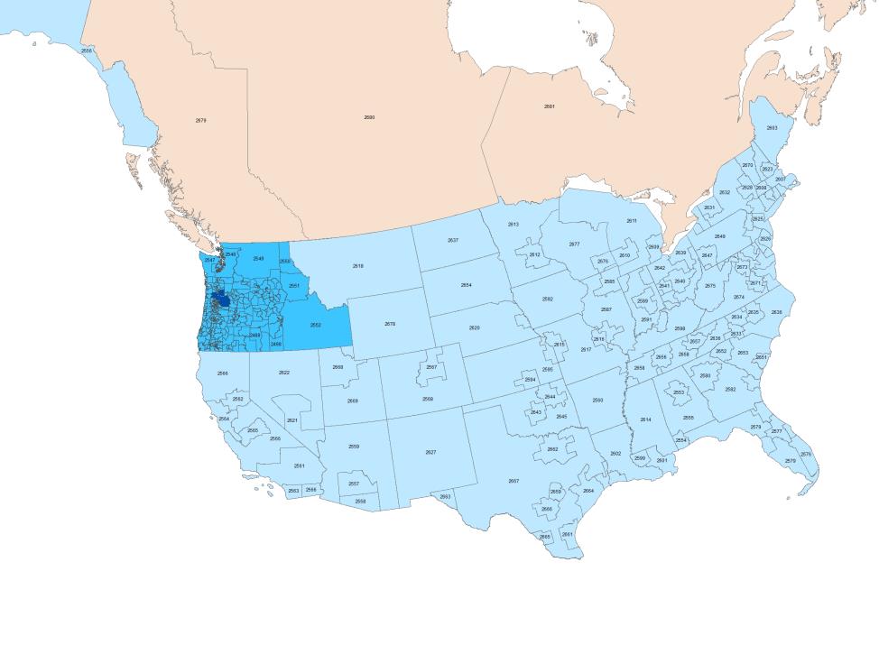

Figure 32. Metro Model Zone System, North American Extent.
Source: (DKS, RSG, and Synergy Associates, 2017)

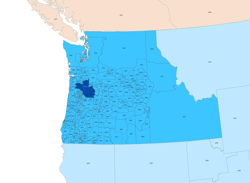
Figure 33. Metro Model Zone System, Oregon and Surrounding States.
Source: (DKS, RSG, and Synergy Associates, 2017)

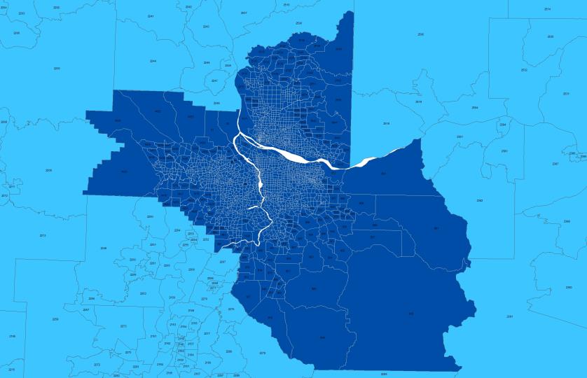
Figure 34. Metro Model Zone System, Metro Model Region.
Source: (DKS, RSG, and Synergy Associates, 2017)

Data Inputs

Metro has collected the following data to support model updates, calibration, and validation of their current truck model:

• FAF commodity flow data, refined by the Port of Portland, through a contractor.
• Gateway truck intercept survey (trucks coming from/to).
• Intercept study of transshipments, which led to a set of rules used for transshipments that were incorporated into their model.
• Ongoing count program, covering trucks though classification counts.

Metro collected data on shipping and truck travel behavior in the region for the development of the new Metro freight model. Metro used an establishment survey that collected both establishment-level data and truck driver diary data. The establishment survey employed both a traditional online survey and a smartphone app. Metro augmented the survey data by acquiring additional GPS truck movement data from INRIX, EROAD, and two businesses with truck fleets in the Portland region.

The Metro freight model uses the following main data sources as input:

• Zone Systems. Uses metro freight model, which combines nationwide FAF zones with TAZs in Oregon, Washington, and Idaho, and more detailed TAZs in the Metro region.
• Economic Data. Includes IO Make and Use tables and industry to commodity correspondences.
• Employment Data. Uses CBP data; Metro employment data by TAZ; LEHD data by Census block for allocation from counties to smaller geographical units.
• Agricultural Census Data. Uses agricultural census data to improve the identification of farms and other agricultural business establishments.
• Commodity Flow Data. Uses FAF4 Data for imports and exports to and from Canada were disaggregated into three Canadian zones.
• Networks. Uses the FAF highway network and Metro's regional travel demand model network for highway skims, with the Metro regional travel demand model used for assignment. Bases the model's nonfreight networks for rail, waterways, and the locations of ports, airports, and intermodal facilities on the NTAD.
• Distribution Centers and Warehouses. Includes a database of the locations of distribution centers and warehouses developed by Metro.

Data Used for Estimating Model Parameters

The Metro freight model used the following main data sources for estimating model parameters:

• Data collected for a national survey as part of the FAME project (Samimi A. M., 2010). Uses these data to estimate the distribution channel model transferred from the earlier CMAP model.
• Commercial vehicle surveys collected in Texas. Uses these data to estimate the shipment sizes model and several of the components of the FTTM, which were transferred from the earlier CMAP model.
• Research conducted by de Jong and Ben-Akiva (de Jong, 2007). Adapts these data to use in the mode and intermediate transfer model to predict the mode and path of long-haul movements of freight based on a comprehensive accounting of transport and logistics costs.
• Ohio General Establishment Survey (Ohio DOT). Uses data from establishment survey to estimate several of the components of the CVTM and FTTM.
• Portland commercial driver diary survey. Uses data from the truck diary survey conducted as part of the project to estimate several of the components of the CVTM and FTTM.
• EROAD dataset for the Portland, Oregon, area. Uses these data to estimate several of the components of the CVTM and FTTM. EROAD is a company that provides onboard vehicle monitoring systems to trucking companies.
• INRIX dataset for the Portland, Oregon, area. Uses these data to estimate several of the components of the CVTM and FTTM. INRIX is a well-known provider of mobility analytical services and smartphone navigation apps.
• Business-specific truck diary datasets. Uses these data to estimate several of the components of the CVTM and FTTM. Two businesses in Portland provided fleet monitoring data for their truck fleets, including similar information to truck diary survey data.

Data Used for Model Calibration and Validation

The calibration and validation of the Metro freight model relied on the following sources:

• Shipment-size distributions from the 2012 CFS.
• Proportions of shipments using direct or complex distribution channels based on the FAME survey.
• Mode choices by commodity and trip type segment (e.g., internal to internal, internal to external) from FAF4.
• Payloads and empty truck proportions from the 2002 VIUS.
• Distributions from the Ohio General Establishment Survey.
• GPS data from combination of truck diary survey, INRIX, EROAD, and business fleets (distributions and O-D data derived by expansion using counts).
• Classified truck counts.

Data Desired, but not Found

Some of the desired—but unobtainable—data for use in the model included the following:

• Detailed data on commodities handled at specific distribution centers, warehouses, and intermodal facilities.
• Data on nonhighway access to specific businesses (e.g., those having rail spurs allowing direct rail deliveries).
• Detailed information about the model and the freight datasets is not yet available online.

SUMMARY

This summary of agency experiences focused on advanced freight forecasting models with elements of supply chain, including firm synthesis, procurement market models, transportation and logistics supply chain models, or truck movement models. This chapter reviewed and summarized seven in-use behavioral supply chain freight models. Table 9 summarizes the models reviewed.

Table 9. Review of Freight Forecasting Models.

Model	Region	Context	Modes Considered (assigned)	Firm Synthesis (model type)	Buyer-Supplier Matching (model type)	Supply Chain Allocation (model type)	Mode and Shipment Size (model type)	Tour-based Truck (model type)	Platform
Chicago	Chicago Metro	Freight	Truck, rail, air, water	Establishment enumeration	Game theory	MNL model	Ben-Akiva and de jong utility equation, MNL model	MNL models, greedy algorithm	R
Florida	State of Florida	Freight	Truck, rail, air, water (truck)	Establishment enumeration	Fuzzy logic	MNL model	Ben-Akiva and de jong utility equation, MNL model	N/A	R
Baltimore/Maryland	Baltimore	Freight and services	Truck, rail, air, water (truck)	Establishment enumeration	Fuzzy logic	MNL model	Ben-Akiva and de jong utility equation, MNL model	MNL models, TSP algorithm, hurdle/count models	R
Portland	Portland Metro	Freight and services	Truck, rail, air, water (truck)	Establishment enumeration	Fuzzy logic	MNL model	Ben-Akiva and de jong utility equation, MNL model	MNL models, TSP algorithm, hurdle/count models	R
Phoenix	Phoenix	Freight and services	Truck, rail, air, parcel (truck)	Establishment evolution	ACE	ACE	Nested Logit	MNL models	R and Java
Oregon	State of Oregon	Integrated model (with CT module)	Truck, rail, air, water, pipeline (truck)	N/A	N/A	N/A	Monte Carlo process	TSP algorithm	R and Java
Wisconsin	State of Wisconsin	Freight and services	Truck, rail, air, water (truck and rail)	Establishment enumeration	Fuzzy logic	Ben-Akiva and de jong utility equation	Ben-Akiva and de jong utility equation	Gravity models	R