Active Transportation and Demand Management (ATDM) Analytical Methods for Urban Streets
CHAPTER 6. SIMULATION EXPERIMENTS
At the outset of the project it was desired to develop a robust active transportation and demand management (ATDM) analytical models based on existing field data, while using simulated data to fill in the gaps. However due to the scarcity of urban street ATDM before-and-after studies located during Task 4 – Existing Data Sources, it became clear that any models developed during this project would need to be based on simulated data, with field data used for validity checks at best. Following the choice of key experimental parameters and testbeds for each active traffic management (ATM) strategy, it was then possible to actually generate the simulated data through simulation experiments. This chapter presents the results of those simulation experiments, which were conducted to meet the requirements of Task 6 – Original Research.
Towards the end of the Task 6 planning phase (end of March 2016), it was decided that the simulation experiments should be geared towards developing capacity adjustment models for each active transportation management (ATM) strategy. This would be consistent with some of the assumptions made during the freeway ATDM project, and consistent with capacity adjustment factors that already exist in the Highway Capacity Manual (HCM). Capacity adjustment models would offer tremendous flexibility in terms of output parameters: they would facilitate the analysis of any performance measure within the HCM urban streets procedure.
DYNAMIC LANE GROUPING CAPACITY ADJUSTMENTS
Due to the nature of the dynamic lane grouping (DLG) experimental conditions, the dynamic lane grouping (DLG) simulation experiments were conducted in the HCS 2010 platform; which is not considered a simulation-based platform, despite containing limited amounts of macroscopic simulation. It is instead primarily an analytical modeling platform, designed to execute the analytical HCM procedures. This platform facilitated the execution of hundreds of signal timing optimizations within a reasonable time frame, as discussed in the previous chapter.
Figure 22 illustrates three of the basic scenarios originally considered for DLG. It was expected that one model would be developed for each scenario. The models could later potentially be unified into a single model with appropriate parameters, if they had enough in common. Because through and right-turn movements on the same intersection approach typically move during the same signal phases, right-turn DLG scenarios were called "100 percent overlap" scenarios. Because through and left-turn movements on the same approach typically move during some but not all of the same signal phases, actuated left-turn scenarios were called "partial overlap" scenarios.
Pre-timed through and left-turn scenarios, in which opposing left-turn phases would terminate
simultaneously, were called "zero overlap" scenarios, because the through and left-turn movements
would never receive green simultaneously. Although traffic analysis tools in the 1990's offered the
ability to model simultaneous termination of opposing left-turn phases at actuated signals, the HCM
2010 procedure did not recognize or support this type of analysis. As such, the "zero overlap"
scenarios were considered a low priority, and were omitted from Task 6 experiments to conserve
project resources.
Note: TH+RT = through and right turn movements. TH+LT = through and left turn movements.
Figure 22. Diagram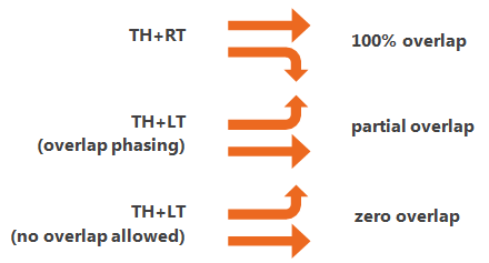 . Phasing scenarios for dynamic lane grouping.
Source: Federal Highway Administration
. Phasing scenarios for dynamic lane grouping.
Source: Federal Highway Administration
Figure 22 illustrates initial data collection efforts for the "partial overlap" model. The "Before" tab of the spreadsheet summarized key input and output parameter values, before DLG was implemented. The "After" tab of the spreadsheet summarized the same values after DLG was implemented. The "Diff" tab automatically computed the ratio of "Before" and "After" results from each cell. "Diff" results were then mapped back to the "Before" tab, to compare DLG impacts against combinations of degree of saturation (v/c) and green ratio (g/C). Similar experiments were conducted for "full overlap" scenarios, and with three exclusive through lanes on the major street. A total of four spreadsheets were created to handle the four combinations of phasing and laneage. These results were then plotted in charts, as shown in Figure 24 and Figure 25.
Blank rows in Figure 23 were the results of scenarios in which intersection delays increased as a result of DLG treatment. Before the Task 6 experiments, it was generally understood that DLG would only be effective in cases where a turning movement was relatively congested, and the adjacent through movement was relatively uncongested. However, the precise ranges where DLG would cease to be effective were unknown. Scenarios where DLG proved ineffective were removed from the charts shown in Figure 24 and Figure 25, in order to make the capacity adjustment results more predictable and stable. It was expected that this would also facilitate development of more accurate capacity adjustment models, later on in Task 6. The plan was to develop "pre-requisite" guidelines for the intersection conditions under which DLG could be effective, and under which the capacity adjustment models would be valid. No models would be needed for predicting DLG impacts under conditions in which DLG was clearly known to be ineffective. These pre-requisite guidelines, based on the data collection results, are presented later in the chapter.
Figure 23 illustrates several of the relevant input and output parameters identified during the experimental planning phase, as described earlier in Chapter 4. Reading from left to right, these include v/c, g/C, capacity (c), and control delay for the through movement; v/c, g/C, capacity (c), and control delay for the left-turn movement; intersection-wide delay; and cycle length. Column K contains the percentage increase in left-turn movement capacity, which resulted from adding a second left-turn lane and re-optimizing the timings. Column F contains the percentage decrease in through movement capacity, which resulted from removing a through lane and re-optimizing the timings.
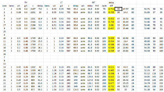 Figure 23. Chart. Data collection results (partial overlap, 2 exclusive through lanes).
Source: Federal Highway Administration
Figure 23. Chart. Data collection results (partial overlap, 2 exclusive through lanes).
Source: Federal Highway Administration
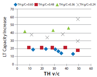
Figure 24 through Figure 27 reflect the original objective of developing capacity adjustment models for both turn movements and through movements, under various congestion levels. These charts were created using the data collected and recorded within spreadsheets, similar to the one shown in Figure 23. The desire to simplify and group results under common g/C values required a trial-anderror signal timing optimization process, as discussed in the previous chapter. Figures 24 and 26 represent the scenarios with three exclusive through lanes on the major street, prior to the removal of a through lane. Figure 25 and 27 represent the scenarios with two exclusive through lanes on the major street. Although these four charts were created for the partial overlap (i.e., left-turn) scenarios, similar charts were created for the full overlap (i.e., right-turn) scenarios.
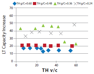 Note: g/C = green time. LT = left turn. TH = through movement. v/c = degree of saturation.
Figure 24. Chart. Left-turn capacity increase (three exclusive through lanes)
Source: Federal Highway Administration
Note: g/C = green time. LT = left turn. TH = through movement. v/c = degree of saturation.
Figure 24. Chart. Left-turn capacity increase (three exclusive through lanes)
Source: Federal Highway Administration
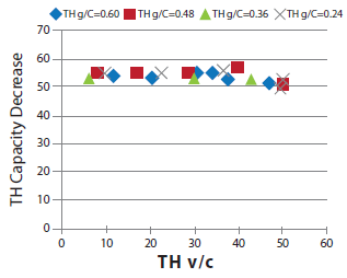
 Note: g/C = green time. LT = left turn. TH = through movement. v/c = degree of saturation.
Figure 25. Chart. Left-turn capacity increase (two exclusive through lanes).
Source: Federal Highway Administration
Note: g/C = green time. LT = left turn. TH = through movement. v/c = degree of saturation.
Figure 25. Chart. Left-turn capacity increase (two exclusive through lanes).
Source: Federal Highway Administration
 Note: g/C = green time. TH = through movement. v/c = degree of saturation.
Figure 26. Chart. Through capacity decrease (three exclusive through lanes)
Source: Federal Highway Administration
Note: g/C = green time. TH = through movement. v/c = degree of saturation.
Figure 26. Chart. Through capacity decrease (three exclusive through lanes)
Source: Federal Highway Administration
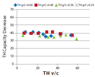
 Note: g/C = green time. TH = through movement. v/c = degree of saturation.
Figure 27. Chart. Through capacity decrease (two exclusive through lanes).
Source: Federal Highway Administration
Note: g/C = green time. TH = through movement. v/c = degree of saturation.
Figure 27. Chart. Through capacity decrease (two exclusive through lanes).
Source: Federal Highway Administration
During this data collection, it was believed capacity adjustment factors or models could soon be developed. This would be similar to what was attempted during the freeway ATDM project. In areas where the data looked unstable, such as in Figure 25, it was hoped that additional data collection would clarify and stabilize those relationships. However, at this point it was realized that even if the capacity adjustment models were perfect, they would nonetheless be unsuitable for arterials. The inadequacy of the capacity adjustment paradigm will now be discussed.
Under the DLG treatment, an exclusive through lane can be temporarily re-channelized as an exclusive left-turn (or right-turn, if needed) lane, to better accommodate fluctuating demands. If that were to happen on the eastbound approach in Figure 28, for example, capacity adjustment models would attempt to predict and re-compute capacities for the eastbound movements. However under actuated or adaptive signal control, this would further affect green times and progression quality for the eastbound left turn, because now its green phase would terminate sooner. It would also re-distribute green time for other movements throughout the signal cycle, possibly altering their capacities and progression quality. If turn pocket queue spillover were alleviated, from a left-turn pocket into an adjacent through lane, multiple movements would again be affected. And as stated both in the previous chapter and in this chapter, signal timings should be re-optimized
whenever lane channelizations change, which would affect movements on all approaches regardless of actuation. The bottom line is that the vehicle flows and green times of all traffic movements at a signalized intersection are highly interdependent, and that prediction of capacity adjustments for one or two movements is not nearly enough to know how the intersection will ultimately operate. In fact, this same concept would hold true for the other relevant ATM strategies in this project, reversible lanes and adaptive signals. Upon this realization, Task 6 efforts were refocused to address the following questions:
- What overall benefits of the ATM strategies are possible under various conditions?
- How can the ATM strategies be implemented within an HCM framework?
These questions will be addressed in the upcoming sub-sections of this chapter.
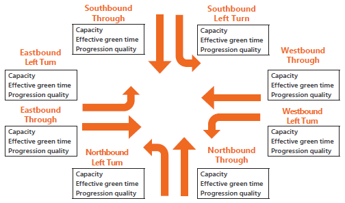 Figure 28. Diagram. Circular dependency of turn movement operations at a traffic signal.
Source: Federal Highway Administration
Figure 28. Diagram. Circular dependency of turn movement operations at a traffic signal.
Source: Federal Highway Administration
ADAPTIVE SIGNAL BENEFITS
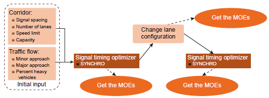
To examine the potential benefits of adaptive signals, the team used the methodology discussed in Chapter 4 (Figure 16) to simulate the three Chicago corridors described in Chapter 4 (Figure 18). The peer review group had expressed concerns about what would be the exact definition of "adaptive signals", and the wide variety of adaptive signal products on the market. The experiment emulated the net result of what an adaptive logic might accomplish, but without using specific commercial adaptive control logic. It was believed that depending on the timing parameters, particularly in terms of creating progression as an "emergent" property, one might obtain very different performance for actuated control. In other words, there is no standard benchmark for actuated control; whereas for pre-timed control, the team used optimized Synchro plans as a baseline. Table 5, Table 6, and Table 7 illustrate the 24-hour impacts of adaptive signals on all three corridors. Although these tables demonstrate consistently positive impacts according to a wide range of performance measures, the magnitudes of these benefits were less consistent (e.g., delay reductions between 3 percent and 24 percent; TTI reductions between 3 percent and 13 percent). The team also simulated the reliability of traffic under rain and snow conditions as follows:
- Randomly select 20 percent of the vehicles traversing any section of the selected locations.
- Perturb their departure time between -5 and +5 minutes.
- Simulate and get the MOEs with and without the strategy.
- Repeat step 1-3 for 20 times using different random seed each time.
- Compute mean and variance of the measures of effectiveness (MOEs).
Table 5. Adaptive signal impacts on West Peterson Avenue (percent change).
| Direction |
Travel Time Index |
Planning Time Index |
Misery Index |
Moving Speed |
Tour Speed |
Delay |
Stop Time |
Stopped Vehicles |
| East |
-1.5 |
1 |
2.7 |
0.7 |
5.4 |
-5.9 |
-5.7 |
-0.6 |
| West |
-33.2 |
-31.9 |
-62.5 |
-0.4 |
4.9 |
-42.9 |
-34.9 |
-1.3 |
| Major |
-8.6 |
-4.2 |
-4.2 |
0.2 |
5.3 |
-13.2 |
-12.5 |
-0.9 |
| Minor |
-3 |
-2.8 |
-0.2 |
1.6 |
5.1 |
-6.8 |
-8 |
-0.6 |
| All |
-3.4 |
-2.3 |
-0.5 |
0.7 |
5.4 |
-5.9 |
-5.7 |
-0.6 |
Table 6. Adaptive signal impacts on West Chicago Avenue (percent change).
| Direction |
Travel Time Index |
Planning Time Index |
Misery Index |
Moving Speed |
Tour Speed |
Delay |
Stop Time |
Stopped Vehicles |
| East |
-17 |
-18 |
-11.7 |
11.9 |
22.4 |
-32.7 |
-28.1 |
-1.2 |
| West |
-2.7 |
-5.8 |
-1.2 |
0.9 |
1.3 |
-6 |
-3.4 |
-1.1 |
| Major |
-16.2 |
-17.9 |
-12.8 |
8 |
13.5 |
-28.8 |
-24.5 |
-1 |
| Minor |
-11.9 |
-8.4 |
-15.4 |
1.8 |
5.4 |
-21.7 |
-25 |
-0.6 |
| All |
-12.7 |
-9.3 |
-13.5 |
2.9 |
7 |
-23.6 |
-24.8 |
-0.7 |
Table 7. Adaptive signal impacts on McCormick Boulevard (percent change).
| Direction |
Travel Time Index |
Planning Time Index |
Misery Index |
Moving Speed |
Tour Speed |
Delay |
Stop Time |
Stopped Vehicles |
| East |
-2.4 |
-4.7 |
-3.1 |
0.9 |
1 |
-10.4 |
-7.7 |
3.4 |
| West |
-43.5 |
-47.7 |
-34.3 |
26.3 |
20.7 |
-30.6 |
-20.4 |
-2.7 |
| Major |
-37.8 |
-54.1 |
-38.9 |
16 |
12 |
-29.5 |
-19.3 |
-0.9 |
| Minor |
-2.4 |
-3.5 |
-1.3 |
0.1 |
1.2 |
-1.5 |
-1.9 |
-0.5 |
| All |
-4.7 |
-6.7 |
-1.8 |
1.1 |
2.1 |
-3 |
-2.7 |
-0.5 |
Experimental conditions corresponded to actually-occurring weather days in Chicago, based on historical records. These experiments indicated that adaptive signal benefits were often more significant under rainy conditions, a finding consistent with (Stevanovic, Zlatkovic, & Dakic, 2015). Rain was found to exhibit the most variability in performance (across the repetitions). By contrast, snow conditions produced a much tighter distribution of performance indicators across repetitions, because speeds were generally very low for all vehicles. Therefore, although adaptive control did not improve average performance under severe weather conditions, it did improve performance reliability under these conditions.
Together with the field study results obtained for Task 4, these simulation results provide the type of data that could potentially be used to develop analytical models for the HCM. However, a number of obstacles still remain. For example, the simulation results demonstrated potential benefits in comparison to an optimized pre-timed plan. Therefore, potential benefits in comparison to an optimized semi-actuated plan are still unknown. Moreover, even if overall benefits compared to semi-actuated control were known, the impact of high-priority input parameters (i.e., Table 3 from Chapter 4) would not be known. In summary, although it should be possible to develop case studies demonstrating the impacts observed during this project, there is still no clear path to developing a generalized adaptive signal model for the HCM, which would accurately handle a wide range of real-world conditions.
REVERSIBLE CENTER LANE BENEFITS
To examine the potential benefits of reversible center lanes (RCL), the team used the methodology illustrated in Figure 29 to analyze hypothetical RCL benefits along the Peterson Avenue corridor described in Chapter 4 (Figure 18). The current operation of Peterson Avenue does not include reversible lanes. In the hypothetical RCL configuration, three lanes were assigned to eastbound traffic, while only one lane was assigned to westbound traffic. Accordingly, the majority of traffic demand was in the eastbound direction. Four different directional demand splits were tested (i.e., 40-60, 30-70, 20-80, and 10-90 percentage split). For example, a 40-60 split implies that 40 percent of traffic flow was in the westbound direction, and 60 percent was in the eastbound direction.
 Note: MOEs = measures of effectiveness
Figure 29. Flowchart. Proposed method for assessing reversible center lane benefits.
Source: Federal Highway Administration
Note: MOEs = measures of effectiveness
Figure 29. Flowchart. Proposed method for assessing reversible center lane benefits.
Source: Federal Highway Administration
As discussed in Chapter 5, degree of saturation was believed to be a critical variable in determining ATM strategy benefits. Thus for each directional split, two demand levels were tested: the original demand level measured in Chicago, and a higher demand level that doubled the original demand. These experimental demand scenarios are shown in Table 8.
Table 8. Demand scenarios for evaluating reversible center lane benefits.
| Demand Vehicles (Vehicles/h) |
High |
Regular |
| Total Volume |
6704 |
3352 |
| Volume Directional Split |
40-60 |
Westbound |
2682 |
1341 |
| Eastbound |
4022 |
2011 |
| 30-70 |
Westbound |
2011 |
1006 |
| Eastbound |
4693 |
2346 |
| 20-80 |
Westbound |
1341 |
670 |
| Eastbound |
5363 |
2682 |
| 10-90 |
Westbound |
670 |
335 |
| Eastbound |
6034 |
3017 |
The experimental results are illustrated through bar charts as shown in Figure 30 and Figure 31. The blue bar represents performance under the base case conditions. The orange bar represents performance under RCL conditions, but before signal timings have been re-optimized. The green bar represents performance under RCL conditions, after signal timings have been re-optimized.
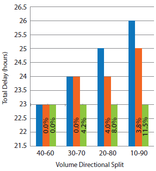 Figure 30. Chart. Reversible center lane delay reductions under original demand levels.
Source: Federal Highway Administration
Figure 30. Chart. Reversible center lane delay reductions under original demand levels.
Source: Federal Highway Administration
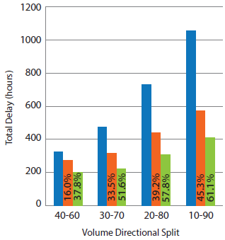 Figure 31. Chart. Reversible center lane delay reductions under heavy demand levels.
Source: Federal Highway Administration
Figure 31. Chart. Reversible center lane delay reductions under heavy demand levels.
Source: Federal Highway Administration
Similar benefits were observed through other performance measures such as vehicle stops, speeds, and travel times. Through these results, it can be concluded that RCL benefits are generally maximized when degrees of saturation and directional splits are both maximized. However the tipping point at which RCL benefits are viewed as significant may depend on a large number of additional factors affecting urban street operations. These could include signal spacing, progression quality, distribution of major/minor-street demands, and corridor reliability. As such, HCM reliability analysis could be an effective method of predicting RCL benefits for a wide variety of urban street conditions. An example HCM reliability analysis of before-and-after-RCL conditions is shown in the next chapter.
DYNAMIC LANE GROUPING BENEFITS
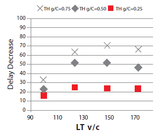
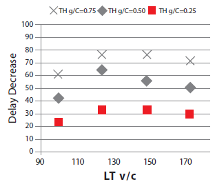
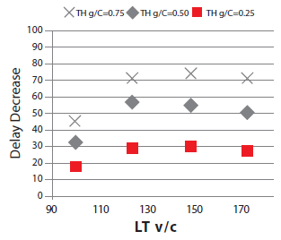
During the initial DLG experiments, it was realized that the interdependent vehicle flows and green times of all signalized traffic movements would make capacity adjustment models impractical. At that time, Task 6 efforts were refocused to address the overall benefits of the ATM strategies under various conditions, and how ATM strategies could be implemented within an HCM framework. As such, new charts were developed from the original DLG data collection efforts described earlier in this chapter. Although the capacity adjustment data collected during those experiments would no longer be useful, the delay reduction data collected during those experiments would now become useful. Figures 32 through 40 illustrate the intersection-wide delay reductions due to DLG, under various conditions.
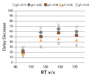
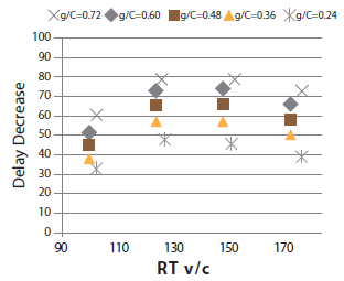 Note: g/C = green time. RT = right turn. v/c = volume to capacity ratio.
Figure 32. Chart. Intersection percentage delay reductions under dynamic lane grouping (right turns, three through lanes, 35 percent degree of saturation for the adjacent through movement).
Source: Federal Highway Administration
Note: g/C = green time. RT = right turn. v/c = volume to capacity ratio.
Figure 32. Chart. Intersection percentage delay reductions under dynamic lane grouping (right turns, three through lanes, 35 percent degree of saturation for the adjacent through movement).
Source: Federal Highway Administration
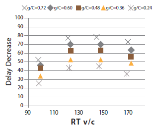 Note: g/C = green time. RT = right turn. v/c = volume to capacity ratio.
Figure 33. Chart. Intersection percentage delay reductions under dynamic lane grouping (right turns, three through lanes, 47 percent degree of saturation for the adjacent through movement).
Source: Federal Highway Administration
Note: g/C = green time. RT = right turn. v/c = volume to capacity ratio.
Figure 33. Chart. Intersection percentage delay reductions under dynamic lane grouping (right turns, three through lanes, 47 percent degree of saturation for the adjacent through movement).
Source: Federal Highway Administration
 Note: g/C = green time. RT = right turn. v/c = volume to capacity ratio.
Figure 34. Chart. Intersection percentage delay reductions under dynamic lane grouping (right turns, three through lanes, 59 percent degree of saturation for the adjacent through movement).
Source: Federal Highway Administration
Note: g/C = green time. RT = right turn. v/c = volume to capacity ratio.
Figure 34. Chart. Intersection percentage delay reductions under dynamic lane grouping (right turns, three through lanes, 59 percent degree of saturation for the adjacent through movement).
Source: Federal Highway Administration
 Note: g/C = green time. RT = right turn. v/c = volume to capacity ratio.
Figure 35. Chart. Intersection percentage delay reductions under dynamic lane grouping (right turns, two through lanes, 30 percent degree of saturation for the adjacent through movement).
Source: Federal Highway Administration
Note: g/C = green time. RT = right turn. v/c = volume to capacity ratio.
Figure 35. Chart. Intersection percentage delay reductions under dynamic lane grouping (right turns, two through lanes, 30 percent degree of saturation for the adjacent through movement).
Source: Federal Highway Administration
 Note: g/C = green time. RT = right turn. v/c = volume to capacity ratio.
Figure 36. Chart. Intersection percentage delay reductions under dynamic lane grouping (right turns, two through lanes, 42 percent degree of saturation for the adjacent through movement).
Source: Federal Highway Administration
Note: g/C = green time. RT = right turn. v/c = volume to capacity ratio.
Figure 36. Chart. Intersection percentage delay reductions under dynamic lane grouping (right turns, two through lanes, 42 percent degree of saturation for the adjacent through movement).
Source: Federal Highway Administration
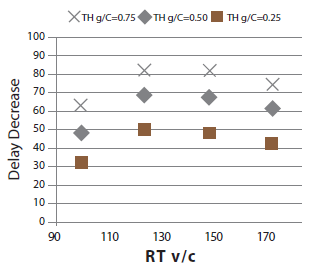
 Note: g/C = green time. LT = left turn. TH = total hours. v/c = volume to capacity ratio.
Figure 37. Chart. Intersection Percentage Delay Reductions under dynamic lane grouping (left turns, three through lanes, 44 percent degree of saturation for the adjacent through movement).
Source: Federal Highway Administration
Note: g/C = green time. LT = left turn. TH = total hours. v/c = volume to capacity ratio.
Figure 37. Chart. Intersection Percentage Delay Reductions under dynamic lane grouping (left turns, three through lanes, 44 percent degree of saturation for the adjacent through movement).
Source: Federal Highway Administration
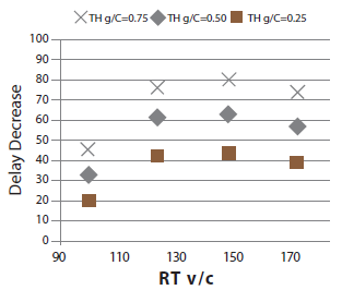
 Note: g/C = green time. LT = left turn. TH = total hours. v/c = volume to capacity ratio.
Figure 38. Chart. Intersection percentage delay reductions under dynamic lane grouping (left turns, three through lanes, 59 percent degree of saturation for the adjacent through movement).
Source: Federal Highway Administration
Note: g/C = green time. LT = left turn. TH = total hours. v/c = volume to capacity ratio.
Figure 38. Chart. Intersection percentage delay reductions under dynamic lane grouping (left turns, three through lanes, 59 percent degree of saturation for the adjacent through movement).
Source: Federal Highway Administration
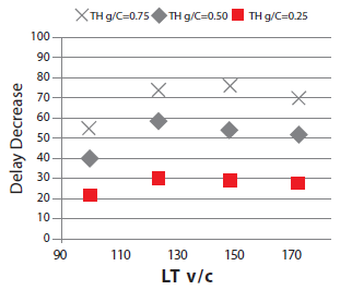
 Note: g/C = green time. LT = left turn. TH = total hours. v/c = volume to capacity ratio.
Figure 39. Chart. Intersection percentage delay reductions under dynamic lane grouping (left turns, two through lanes, 30 percent degree of saturation for the adjacent through movement).
Source: Federal Highway Administration
Note: g/C = green time. LT = left turn. TH = total hours. v/c = volume to capacity ratio.
Figure 39. Chart. Intersection percentage delay reductions under dynamic lane grouping (left turns, two through lanes, 30 percent degree of saturation for the adjacent through movement).
Source: Federal Highway Administration
 Note: g/C = green time. LT = left turn. TH = total hours. v/c = volume to capacity ratio.
Figure 40. Chart. Intersection percentage delay reductions under dynamic lane grouping (left turns, two through lanes, 42 percent degree of saturation for the adjacent through movement).
Source: Federal Highway Administration
Note: g/C = green time. LT = left turn. TH = total hours. v/c = volume to capacity ratio.
Figure 40. Chart. Intersection percentage delay reductions under dynamic lane grouping (left turns, two through lanes, 42 percent degree of saturation for the adjacent through movement).
Source: Federal Highway Administration
A small number of additional experiments were performed with shared lane scenarios, and
with right-turns-or-red (RTOR) allowed. In a shared lane scenario, lane channelization can be
dynamically changed from shared to exclusive, or vice-versa. Also, it is not uncommon for the
inside right-turn lane of a dual right-turn lane group to have RTOR allowed. These experiments
found that shared lane DLG produces no significant benefits for right turns unless RTOR is
allowed, and produces no significant benefits for left turns. However in shared lane RTOR cases
where DLG produces significant benefits, those benefits would be very hard to predict by a simple
method or chart, due to the sheer number of independent variables (e.g., conflicting through (TH) demand,
opposing left turn (LT) demand, existence of shielded right turn (RT) phase, v/c of multiple movements, g/C of multiple
movements).
Following the production of these delay reduction charts, the following observations became possible:
- Significant benefits only occur when turn movement degree of saturation (v/c) exceeds 95 percent; and when adjacent through movement degree of saturation is at least 5 percent lower than (N-1)/N, where N is the number of exclusive through lanes prior to DLG.
- Benefits are much higher when g/C is high on the DLG approach prior to DLG (in other words, when DLG movements receive green during most of the cycle prior to DLG).
- Benefits are increased when turn movement degree of saturation is in the mid-100-percent range, prior to DLG (in other words, when adding a new turn lane allows the turn movement to go from significantly oversaturated to undersaturated).
- Benefits are increased when cycle lengths can be re-optimized to accommodate the new lane grouping (may not be effective with other congested intersections in the urban street, which may govern the background cycle length).
- Similar benefits are observed for left turns versus right turns, and for two exclusive through lanes versus three exclusive through lanes (however, the pre-requisite listed in the first bullet may be harder to satisfy with only two exclusive through lanes).
- Benefits increase when there is good progression quality on the DLG approach, prior to DLG (observed in bonus experiments where "arrival types" were modified in HCS 2010).
- If it were possible to automatically detect v/c and g/C of various turn movements, it might become more effective to implement DLG in real time than by fixed time-of-day.
CONCLUSIONS AND NEXT STEPS
An initial set of simulation experiments was geared towards the development of capacity adjustment models for three ATM strategies. After a few weeks of these experiments, it became apparent that vehicle flows and green times of all traffic movements at a signalized intersection are highly interdependent, and that capacity adjustment for one or two movements could not accurately predict intersection operations. In fact, this same concept would hold true for all relevant ATM strategies in this project. Upon this realization, Task 6 efforts were refocused to address the following questions:
- What overall benefits of the ATM strategies are possible under various conditions?
- How can the ATM strategies be implemented within an HCM framework?
Potential overall benefits under various conditions were partially addressed by experimental results presented in the second and third sub-sections of this chapter. However the next step, and a crucial component of this project, would be the issue of how ATM strategies could be implemented in an HCM framework. The next chapter will address this issue by demonstrating how some ATM strategies can be implemented within an HCM framework. These implementations can also further address the first bulleted question, regarding potential ATM strategy benefits. In fact, these HCM implementations may make it easier to determine ATM strategy benefits under various conditions, without requiring simulation studies. This was an original and primary goal of the project.