Active Transportation and Demand Management (ATDM) Analytical Methods for Urban Streets
CHAPTER 7. HIGHWAY CAPACITY MANUAL FRAMEWORK IMPLEMENTATION
In the early stages of the project, it was believed that the three chosen urban street active traffic management (ATM) strategies could be effectively modeled via capacity adjustment factors, similar to what was accomplished during the freeway active transportation and demand management (ATDM) project. However, it was later discovered that the capacity adjustment paradigm would be unsuitable for arterials, and that the Highway Capacity Manual (HCM) reliability framework would offer a preferable solution. Specifically, the alternative lane use configurations could be modeled as special event datasets within the HCM reliability framework, along with re-optimized timing plans for the new lane uses. The inadequacy of the capacity adjustment paradigm was detailed in the previous chapter.
The research team was always aware of the ability to model alternative lane use configurations as special event datasets within the HCM reliability framework. However, the team had hoped that capacity adjustment models might provide another modeling option. Capacity adjustment models (or factors) would have made it possible for engineers to analyze ATM strategy impacts without having to develop alternative datasets, and without having to develop alternative optimized timing plans. Access to both modeling options would have provided great flexibility for the analyst, just as simulation and the HCM provide alternate modeling options for many facility types. Thus when the capacity adjustment option was deemed inadequate, the HCM reliability framework quickly became the best and only option for ATM strategy.
RELIABILITY FRAMEWORK FUNDAMENTALS
The HCM reliability framework is largely based on the product of a second Strategic Highway Research Program (SHRP 2) project (Zegeer, et al., 2014). At its core, the reliability methodology consists of hundreds of repetitions of the HCM urban streets methodology. In contrast to the urban streets methodology, where inputs represent average values for a defined analysis period, the reliability methodology varies the demand, capacity, geometry, and traffic control inputs to the facility methodology with each repetition (i.e., scenario). Chapter 17 of the recently-published HCM 6th Edition provides the following additional description:
The full range of HCM performance measures output by the facility methodology are assembled for each scenario and used to describe the facility's performance over the course of a year (or other user-defined reliability reporting period). Performance can be described on the basis of a percentile result (e.g., the 80th or 95th percentile travel time) or
the probability of achieving a particular level of service (e.g., the facility operates at LOS D during X percent of weekday hours during the year). Many other variability and reliability performance measures can be developed from the
facility's travel time distribution.
The reliability methodology is sensitive to the main sources of variability that lead to travel time unreliability. These sources are identified in the following list.
- Temporal variability in traffic demand—both regular variations by hour of the day, day of the week, and month or season of the year and random variations between hours and days.
- Incidents that block travel lanes or that otherwise affect traffic operations and thus capacity.
- Weather events that affect capacity and possibly demand.
- Work zones that close or restrict travel lanes, thus affecting capacity.
- Special events that produce atypical traffic demands that may require management by special traffic control measures.
Figure 41 further illustrates the reliability framework described above. The analyst must define their desired study period and study section in advance. Within the resulting "analysis box," a certain proportion of "cells" could potentially benefit from ATM strategies, depending on their traffic operational conditions. In this case, the occurrence of an ATM strategy activation could be considered a special event, and could be modeled accordingly.
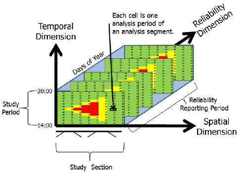 Figure 41. Image. Reliability analysis box.
Source: (Transportation Research Board of the National Academies, 2010)
Figure 41. Image. Reliability analysis box.
Source: (Transportation Research Board of the National Academies, 2010)
RELIABILITY FRAMEWORK DATASETS
The input data needed to evaluate an HCM urban street for one analysis period can be referred to as a "dataset." However for evaluations involving special events or work zones, the reliability framework requires more than one HCM dataset. The "base" dataset describes base conditions when work zones and special events are not present, and can represent average conditions. As implied earlier, the reliability framework essentially generates hundreds of copies of the base dataset. This allows these hundreds of scenario datasets to have their inputs adjusted to reflect varying demands, weather, incidents, and other time-varying conditions throughout the year.
Although the HCM reliability framework contains procedures for intelligently adjusting traffic volume, saturation flow rate, free-flow speed, capacity, and other inputs to reflect time-varying conditions throughout the year, some time-varying conditions are too complex or unpredictable for the procedure to handle on its own. "Alternative" datasets are needed to describe conditions when a specific work zone is present, or when a special event occurs. For example, if a large sporting event affects 3 percent of cells within the annual analysis, an alternative dataset reflecting those
conditions would be applied to generate the results for those cells. This alternative dataset may have lane geometries, signal timings, free-flow speeds, and saturation flow rates that deviate significantly from the base dataset, such that only an engineer familiar with local conditions could accurately specify them.
ACTIVE TRAFFIC MANAGEMENT STRATEGY IMPLICATIONS
The paradigm of alternative datasets within the HCM reliability framework is the way in which ATM strategies can be modeled. For example, an alternative dataset for the dynamic lane grouping (DLG) strategy might have two exclusive right-turn lanes instead of one, two exclusive through lanes instead of three, and signal timings re-optimized to accommodate the new lane use. Similarly, an alternative dataset for reversible center lanes might have an additional exclusive through lane at all intersections in the westbound direction, one fewer exclusive through lane at all intersections in the eastbound direction, and signal timings re-optimized to accommodate the new lane uses. In this manner, as long as the alternative datasets were applied during the proper time periods, the overall reliability model could be accurate and effective. For DLG, the pre-requisite criteria developed in the previous chapter provide possible guidance in selecting time periods in which DLG could be effective. For reversible lanes, a simpler analysis of directional demands (e.g., through the ARTPLAN tool) could reveal optimum time periods for implementation. The potential for modeling adaptive signals in this manner is less clear. Alternate lane groupings and center lane reversals are typically in effect throughout multiple 15-minute time periods before reverting to the original lane geometries, which is consistent with typical HCM modeling. By contrast, adaptive signals produce significant signal timing changes as frequently as every minute, or every two minutes. Furthermore, adaptive signals are known to produce significant inefficiencies during their "transition" periods (Pohlmann & Friedrich, 2014), and the HCM framework might not capture these transition effects. Transition effects also exist for alternate lane groupings and center lane reversals; but because these transitions occur with so much less frequency, their impacts on yearly, daily, and perhaps even hourly overall results, are negligible.
HIGHWAY CAPACITY MANUAL FRAMEWORK CASE STUDIES
Chapter 3 introduced the available software platforms for HCM urban street reliability analysis: Streetval-Java and HCS-Streets. If special event modeling (via alternate datasets) can be successfully implemented within one or both of these platforms, it would then become possible to assess ATM impacts in terms of annual reliability and other advanced measures. Although efforts are underway to implement special event modeling within these platforms, this functionality is not yet ready for testing. Therefore, the only current way to assess ATM impacts in the reliability framework is by testing two different base datasets: one base dataset with the ATM treatment, and one base dataset without the ATM treatment. Because of this limitation, the reliability analysis box will be limited to the time periods where ATM treatments are effective. Note that this may cause the benefits to appear exaggerated. If it were possible to test these ATM strategies through special event modeling, the annual benefits would be more modest, because many time periods do not require ATM treatments.
In this project, dynamic lane grouping and reversible center lanes were tested within the HCM reliability framework. This testing was performed within the HCS-Streets platform. Results from these two case studies are presented in the following sub-sections. To reiterate, the reliability analysis box will be limited to time periods in which ATM treatments are effective, which may cause the benefits to appear exaggerated.
The purpose of these case studies is to provide a proof-of-concept, which demonstrates how certain ATM strategies can be implemented within the HCM reliability framework. Although some ATM strategies (e.g., adaptive signals) may not fit within the framework without additional research and development, other strategies are modeled more readily through modification of HCM datasets. An ideal case study would clearly demonstrate ATM strategy benefits for typical urban street conditions.
To establish such typical conditions, an example dataset from HCM 6th Edition Chapter 30 (Urban Street Segments: Supplemental) was used as a baseline. This urban street has two exclusive through lanes on the major street, but only one on the minor street. Baseline intersection spacings are illustrated in Figure 42. Baseline volume demands are illustrated in Figure 43. The fundamental characteristics (e.g., traffic volume demands, lane channelizations, signal timings) of this dataset provide a good starting point for analysis of typical conditions, but several important adjustments were still needed. Specifically, there was a need to introduce:
- Typical intersection spacings that would benefit from signal timing coordination.
- Time-varying demands across multiple time periods.
- Oversaturation within the "middle" time periods.
- Directional splits (i.e., significantly heavier volume demands on one of the two major-street directions).
- Turn movement demands that would reflect a need for ATM interventions, while simultaneously falling within the umbrella of typical urban street conditions.
- Signal timings re-optimized to best accommodate all of these changes.
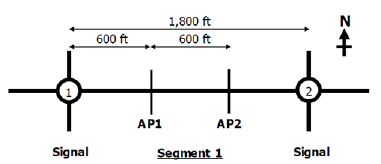 Figure 42. Diagram. Baseline intersection spacing.
Source: Transportation Research Board of the National Academies, 2010
Figure 42. Diagram. Baseline intersection spacing.
Source: Transportation Research Board of the National Academies, 2010
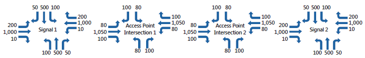 Figure 43. Diagram. Baseline traffic volumes
.
Source: Transportation Research Board of the National Academies, 2010
CASE STUDY #1: DYNAMIC LANE GROUPING
The case studies for DLG and reversible center lanes will each describe a customization of input conditions, summary of output results, and interpretation of output results.
Intersection Spacings
In the example dataset from HCM Chapter 30 there are two signalized intersections, and two mid- block access points. The distance between the signalized intersections is 1800 feet. At this distance, platoon progression benefits are minimal, and signal coordination benefits are minimal. To create case study conditions more sensitive to platoon progression and signal coordination, the distance between signals was reduced to 500 feet, and the access points were eliminated. It was believed that the 500-foot spacing with no access points would help to reveal DLG impacts more clearly.
Time-Varying Demands
In typical real-world conditions, traffic volume demands continuously fluctuate throughout each hour. The HCM recommends 15-minute time periods for capturing the impacts of these changes. The Manual further recommends that when analyzing oversaturated conditions, both the first and final time periods should be undersaturated, so that residual queuing can be fully addressed within the "middle" time periods. This is why the congested red area is fully contained within the analysis box, as shown in Figure 41 earlier. Since analysis of oversaturated traffic conditions is believed
to be a top national priority, the case study dataset was split up into four 15-minute time periods, with degrees of saturation exceeding 100 percent for some turn movements during time period #2. Specific volume demand modifications are listed below:
- Time period #1: turn movement volumes unchanged at both intersections.
- Time period #2: turn movement volumes increased by 20% at both intersections.
- Time period #3: turn movement volumes decreased by 10% at both intersections.
- Time period #4: turn movement volumes decreased by 10% at both intersections.
This creation of time-varying demands causes residual queues to form during time period #2, dissipate during time period #3, and further dissipate during time period #4. Despite time periods #3 and #4 having the same traffic volume demands, delays and queue lengths are actually lighter in time period #4 relative to time period #3, because the congestion from time period #2 has had more time to dissipate. This is believed to be more representative of the typical congested conditions that need to be addressed in developed nations. If DLG and other ATM strategies can effectively mitigate such conditions, then these strategies will be valuable.
Directional Splits
In typical real-world conditions, directional traffic demands are significantly unbalanced during peak time periods. In the AM peak period, the vast majority of commuters travel into or towards some sort of city center, or central business district. In the PM peak, most drivers travel in the opposite direction. It is this commuting demand that places the greatest strain upon transportation networks, and creates a need for ATM strategies.
In the example dataset from HCM Chapter 30, baseline traffic volume demands are illustrated in Figure 43. It can be seen that traffic demands are identical along both major-street (eastbound and westbound) directions. As such, the baseline demands are not representative of top-priority traffic congestion problems that need to be solved, and do not reflect typical peak period conditions. To remedy this, the following directional volume adjustments were made:
- Eastbound turn movement volumes increased by 10 percent at both intersections during all time periods.
- Westbound turn movement volumes decreased by 10 percent at both intersections during all time periods.
This created a 20 percent directional split (i.e., 60:40) along the major-street direction. Benefits were then analyzed for DLG in the heaviest (i.e., 60 percent) direction of traffic. According to the Chapter 5 findings, benefits increase when there is good progression quality on the DLG approach, prior to DLG treatment. This would not preclude DLG from ever being beneficial in the lightest direction of travel, although in those cases benefits could be less significant
Demands Requiring Active Traffic Management Intervention
Following the adjustments for time-varying demands and directional splits, additional demand adjustments were needed to assess potential ATM benefits. This is because, as shown in Figure 43 earlier, through movement demands greatly exceed their adjacent turn movement demands, as is typical on urban streets. Although this distribution of turn movement demands is typical, a sharp increase in right-turn (or left-turn) demands during certain time periods is not uncommon. This could be caused by a special attractor, such as a post office that drivers must visit on their way home, or a church that receives heavy traffic on weekends. Regardless of the reason for heavy turn movement demands in certain time periods, the DLG treatment is designed to accommodate those sharply changing demands.
Referring to Figure 42 and Figure 43 earlier, eastbound through and left-turn volumes were changed at intersection #2 for this experiment. Specifically, eastbound left-turn volumes were increased by 100 vehicles per hour (veh/h) in all time periods at intersection #2. At the same time, eastbound through volumes were decreased by 100 vehicles per hour (veh/h) in all time periods at intersection #2. Figure 44 illustrates these changes. Despite the left-turn demands never exceeding their adjacent through movement demands in any time period, the restrictive nature of left-turn signal phases caused left-turn degrees of saturation to greatly exceed their adjacent through movement demands in every time period, even when signal timings were optimized. These are the pre-requisite conditions for DLG effectiveness, as discussed in the prior chapters.
Figure 44. Diagram. Creation of demands requiring dynamic lane grouping treatment.
| Movement |
Before |
After |
| Left Turn - Time Period #1 |
55 |
155 |
| Left Turn - Time Period #2 |
66 |
166 |
| Left Turn - Time Period #3 |
50 |
150 |
| Left Turn - Time Period #4 |
50 |
150 |
| Through - Time Period #1 |
275 |
175 |
| Through - Time Period #2 |
330 |
230 |
| Through - Time Period #3 |
250 |
150 |
| Through - Time Period #4 |
250 |
150 |
Note: all volumes in units of vehicles per hour.
Source: Federal Highway Administration
Re-Optimized Signal Timings
Following the aforementioned changes involving signal spacings and demand volumes, it was appropriate to re-optimize signal timings (i.e., cycle length, green splits, offsets) for both intersections. Phasing sequence optimization was omitted from this process, but phasing sequence was unlikely to have a significant impact under these conditions. This re-optimization effort was appropriate because in practice, local engineers would often not allow obsolete signal timings to remain in effect after a fundamental change in lane groupings.
In the HCS 2010 platform, signal timings are optimized via genetic algorithm (Hale, Park, Stevanovic, Su, & Ma, 2015) (Park, 1998) (Agbolosu-Amison, Park, & Yun, 2009). In this case study, "Overall Delay" was chosen as the optimization objective function. Figure 45 illustrates the time-period specific degrees of saturation at intersection #2, before and after the eastbound flows were increased (left turns) and decreased (through movements) to warrant DLG treatment. Figure 45 degrees of saturation in the "after" column also reflect the re-optimized signal timings. Without the re-optimization effort, degrees of saturation would have been much higher in the "after" column. Another impact of the re-optimization effort was that the urban street cycle length increased from 117 seconds to 127 seconds, in order to accommodate the increased congestion.
Figure 45. Diagram. Degrees of saturation before and after eastbound volume changes.
| Movement |
Before |
After |
| Left Turn - Time Period #1 |
86% |
129% |
| Left Turn - Time Period #2 |
86% |
159% |
| Left Turn - Time Period #3 |
85% |
104% |
| Left Turn - Time Period #4 |
85% |
104% |
| Through - Time Period #1 |
76% |
47% |
| Through - Time Period #2 |
99% |
76% |
| Through - Time Period #3 |
62% |
36% |
| Through - Time Period #4 |
62% |
36% |
Source: Federal Highway Administration
Given the sharp contrasts between left-turn and through movement degrees of saturation, conditions were now ripe to perform a before-and-after analysis, in which the "after" analysis would convert the leftmost through lane into a second exclusive left-turn lane. Figure 46 illustrates the time-period specific degrees of saturation at intersection #2, before and after DLG treatment. Figure 46 degrees of saturation in the "after" column also reflect yet another re-optimization of signal timings, in which the background cycle length decreased from 127 seconds to 120 seconds. These results
show that through movement operations were being compromised to relieve left-turn movement congestion, in a way that substantially lowers overall intersection delays. The intersection-wide and corridor-wide benefits will be illustrated later.
Figure 46. Diagram. Degrees of saturation before and after dynamic lane grouping
| Movement |
Before |
After |
| Left Turn - Time Period #1 |
129% |
89% |
| Left Turn - Time Period #2 |
159% |
97% |
| Left Turn - Time Period #3 |
104% |
86% |
| Left Turn - Time Period #4 |
104% |
87% |
| Through - Time Period #1 |
47% |
91% |
| Through - Time Period #2 |
76% |
133% |
| Through - Time Period #3 |
36% |
70% |
| Through - Time Period #4 |
36% |
70% |
Source: Federal Highway Administration
Reliability Analysis
In order to perform the before-and-after reliability analysis, it was necessary to first define the reliability analysis box within HCS 2010. Spatial limits were already defined within the base dataset. Regarding temporal limits of the analysis, these limits were defined as January 1st 2015 through January 1st 2016. However, only Tuesdays, Wednesdays, and Thursdays would be included in the analysis. This produced a total of 157 analysis days. Given that there were four time periods in the base dataset, this led to the creation of 157*4 = 628 total scenarios. Weather impacts were automatically imported from the Washington DC area. Default hourly, weekly, and monthly demand volume distributions within the software were accepted. It was assumed that the corridor would experience no traffic accidents.
The overall results are illustrated in Figure 47 and Figure 48. These results show that DLG decreased total delay by 39 percent (i.e., from 32.7 to 19.9 vehicle-hours), which accounts for all approaches at both intersections. However the results also show that corridor travel time more than doubled (i.e., from 35 to 75 seconds), reflecting sacrifices made by the through movements. This implies that decisions over whether to implement DLG should depend on local priorities, and to what extent through vehicles should receive preferential treatment over turning vehicles. Finally, reliability measures such as TTI and PTI are also provided by HCS 2010.
This case study showed that DLG could be explicitly analyzed within the HCM reliability framework, and could provide significant operational benefits. The exercise also demonstrates that perhaps not all time periods need to satisfy the pre-requisite criteria suggested in Chapter 5. There it was stated that significant benefits only occur when adjacent through movement degree of saturation is at least 5 percent lower than (N-1)/N (where N is the number of exclusive through lanes), prior to DLG treatment. However DLG was highly beneficial here, despite time period #2 clearly violating this pre-requisite. Finally, when considering the impressive 39 percent delay reduction, it should be remembered that benefits may be exaggerated by a reliability analysis box confined to ATM-friendly time periods, as mentioned earlier in the chapter.
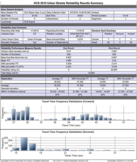 Figure 47. Image. Reliability analysis results before dynamic lane grouping.
Source: McTrans Center, University of Florida
Figure 47. Image. Reliability analysis results before dynamic lane grouping.
Source: McTrans Center, University of Florida
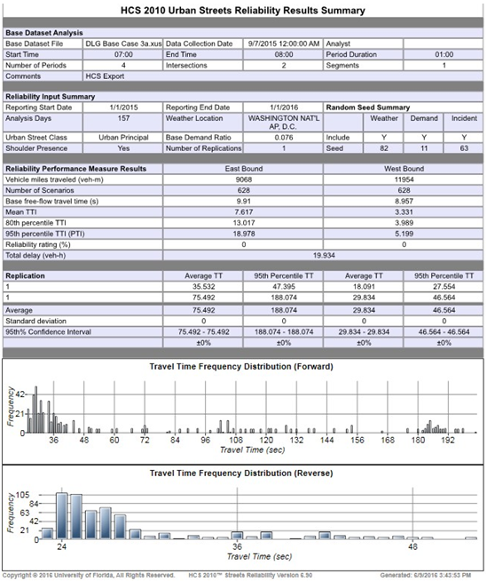 Figure 48. Image. Reliability analysis results after dynamic lane grouping.
Source: McTrans Center, University of Florida
Figure 48. Image. Reliability analysis results after dynamic lane grouping.
Source: McTrans Center, University of Florida
CASE STUDY #2: REVERSIBLE CENTER LANES
Similar to the prior case study for DLG, case study #2 for reversible center lanes (RCL) will describe a customization of input conditions, summary of output results, and interpretation of output results.
Corridor Geometry
For reasons discussed in the prior case study, the distance between signals was reduced to 500 feet, and the access points were eliminated. However to simplify the analysis, left- and right-turn movements were eliminated at all intersections. This was because major-street left turns are often prohibited along RCL corridors, and because minor-street demands could be easily modified
without introducing flow-balancing discrepancies along the major street. Left-turn volume demands were added and combined into the through movement demands. Right-turn volume demands were deleted from the analysis.
Time-Varying Demands
For reasons discussed in the prior case study, the RCL case study dataset was split up into four 15-minute time periods, with eastbound degrees of saturation exceeding 100 percent during time period #2. Specific volume demand modifications are listed below:
- Time period #1: volumes decreased by 20 percent at both intersections.
- Time period #2: volumes unchanged at both intersections.
- Time period #3: turn movement volumes decreased by 25 percent at both intersections.
- Time period #4: turn movement volumes decreased by 25 percent at both intersections.
Due to the absorption of left-turn demands into the through movement, significant new congestion was created. As such, volumes were not increased as much during this stage as they were during the parallel DLG stage. As with the prior case study, this creation of time-varying demands caused residual queues to form during time period #2, dissipate during time period #3, and further dissipate during time period #4. Despite time periods #3 and #4 having the same traffic volume demands, delays and queue lengths were again lighter in time period #4 relative to time period #3, because the congestion from time period #2 had more time to dissipate. This is believed to be more representative of typical congested conditions, and any ATM strategy capable of mitigating such conditions would be valuable.
Directional Splits Requiring Active Traffic Management Intervention
Efficient handling of significant directional splits provides the impetus behind the RCL strategy. As discussed in the prior case study, directional traffic demands are typically very unbalanced during peak time periods, due to typical commuting patterns. In the example dataset from HCM Chapter 30, baseline traffic volume demands were illustrated in Figure 42. It can be seen that traffic demands are identical along both major-street (eastbound and westbound) directions. These baseline demands are not representative of top-priority traffic congestion problems, and do not reflect typical peak period conditions. To remedy this, the following directional volume adjustment was made:
- Westbound volumes decreased by 20 percent at both intersections during all time periods.
This created a 20 percent directional split (i.e., 60:40) along the major-street direction. The case study would then attempt to assess RCL benefits for this 60:40 split. Benefits of RCL would potentially be greater for 70:30 and 80:20 directional splits, which are not uncommon. In the "before" scenario, only one exclusive through lane would serve the critical eastbound direction. This reflects a typical scenario in which lane use was designed to accommodate the highest daily demand direction (e.g., PM peak), but then is much less efficient during the second highest demand direction (e.g., AM peak). In the "after" scenario, one exclusive through lane would be donated from the westbound direction to the eastbound direction.
Re-Optimized Signal Timings
Following the above changes, it was appropriate to re-optimize signal timings (i.e., cycle length, green splits, offsets) for both intersections. Phasing sequence optimization was again omitted from the process, and "Overall Delay" was again chosen as the objective function. This re-optimization effort was appropriate because local engineers would typically not allow obsolete signal timings to remain in effect, after a change in lane use. Given the sharp contrast in the number of exclusive through lanes available to each major-street direction, conditions were now ripe to perform a before-and-after analysis in which the "after" analysis would convert one westbound through lane into an eastbound through lane. Figure 49 illustrates the time-period-specific degrees of saturation before and after RCL treatment. Figure 49 degrees of saturation in the "after" column reflect yet another re-optimization of signal timings, in which the background cycle length decreased from 103 seconds to 70 seconds. These results show that westbound operations were being compromised to relieve eastbound congestion, in a way that substantially lowered overall corridor travel times.
The corridor-wide benefits will be illustrated later.
Figure 49. Diagram. Degrees of saturation before and after reversing center lanes.
| Movement |
Before |
After |
| Eastbound Through - Time Period #1 |
90% |
51% |
| Eastbound Through - Time Period #2 |
100% |
54% |
| Eastbound Through - Time Period #3 |
77% |
44% |
| Eastbound Through - Time Period #4 |
77% |
44% |
| Westbound Through - Time Period #1 |
38% |
78% |
| Westbound Through - Time Period #2 |
50% |
109% |
| Westbound Through - Time Period #3 |
32% |
65% |
| Westbound Through - Time Period #4 |
32% |
65% |
Source: Federal Highway Administration
Reliability Analysis
In order to perform the before-and-after reliability analysis, it was necessary to first define the reliability analysis box within HCS 2010. These reliability parameters were the same as those used during the DLG case study. Spatial limits were defined in the base dataset. Temporal limits were again defined as January 1st 2015 through January 1st 2016. Only Tuesdays, Wednesdays, and Thursdays were included in the analysis. This produced a total of 157 analysis days and 157*4 = 628 total scenarios. Weather impacts were imported from the Washington DC area. Default hourly, weekly, and monthly demand volume distributions within the software were accepted. It was assumed that the corridor would experience no traffic accidents.
The overall results are illustrated in Figure 50 and Figure 51. These results show that RCL decreased total delay by 30 percent (i.e., from 8.1 to 5.6 vehicle-hours), which accounts for all approaches at both intersections. However the results also show that corridor travel time increased slightly, from 18.5 to 20.1 seconds. This is likely due to the "Overall Delay" objective function, which often mitigates side-street delays at the expense of arterial progression. Finally, reliability measures such as TTI and PTI also reflect slightly higher travel times when RCL is in effect.
This again probably has more to do with the optimization objective function than with the RCL treatment itself. In fact, when "Travel Time" and/or "Arterial Delay" were tried as the objective functions in subsequent test optimizations, the result both times was a five-minute cycle length, and only five seconds of green time on the minor street, producing overwhelming amounts of delay on the side street. Therefore, the original 30 percent delay reduction achieved by the "Overall Delay" objective function was probably the best attainable result in this software platform, despite the modest increase in major-street travel times.
This case study showed that RCL could be explicitly analyzed within the HCM reliability framework, and could provide significant operational benefits. The exercise also demonstrated the difficulty in reconciling conflicting objectives such as minimizing overall delays, and minimizing major-street travel times. Finally, when considering the 30 percent delay reduction, it should be remembered that benefits may be exaggerated by a reliability analysis box confined to ATM-friendly time periods, as mentioned earlier in the chapter.
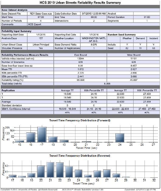 Figure 50. Image. Reliability analysis results before reversing center lanes.
Source: McTrans Center, University of Florida
Figure 50. Image. Reliability analysis results before reversing center lanes.
Source: McTrans Center, University of Florida
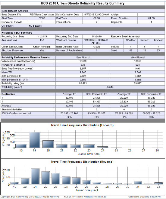 Figure 51. Image. Reliability analysis results after reversing center lanes.
Source: McTrans Center, University of Florida
Figure 51. Image. Reliability analysis results after reversing center lanes.
Source: McTrans Center, University of Florida
CONCLUSIONS
In the early stages of the project, it was believed that the chosen urban street ATM strategies could be effectively modeled via capacity adjustment factors. However, it was discovered that this would be unsuitable for arterials, and that the HCM reliability framework would offer a preferable solution. At that point, the HCM reliability framework quickly became the best and only option for ATM strategy implementation. Two case studies performed in the HCS 2010 reliability engine, for dynamic lane grouping and reversible center lanes, provided a proof-of-concept for ATM strategies implementation within the HCM reliability framework. It is not clear whether adaptive signals or other advanced ATDM strategies could be accurately analyzed in this manner.