Safety Implications of Managed Lane Cross Sectional ElementsCHAPTER 5: ANALYSISStatistical Model / MethodologyBecause more than one time period from each site was used as an analysis unit, the statistical methodology had to consider the grouping structure in the data in an explicit manner. Generalized Linear Mixed models can account for such a structure, as well as handling fixed effects, the type of parametric estimation expected to yield answers to the research questions. These models are constructed under the assumption that crashes at study sites for a given time period follow a given probability distribution. Depending on the dispersion of a particular subset of data, this work utilized Poisson or Negative Binomial distributions. In the case of the Poisson log-linear mixed effects model, the probability distribution is as shown in Figure 10. Figure 10. Equation. Probability distribution. Where: The expected number of crashes at the ith site is simply Although most time periods were one-year long, the methodology allows the incorporation of partial years, as this variable is handled as exposure in a way similar to segment length. The exposure variables in the model are defined as the product of the time period length (expressed in years) and the segment length (expressed in miles) for each record in the database. This quantity has units of mile-years (mi-yr). For a given segment-period with amount of exposure Figure 11. Equation. Initial equation. Where: Since The exponential function is used to parameterize the quantity Figure 12. Equation. Equation with crashes per mile-year for ith site. Where: As indicated by the sub-index, the model computes a unique Figure 13. Equation. Equation with model random effect distribution. Where: The statistical analysis estimates the quantities Overview Of Variables ConsideredInitially, variables were selected based on the findings of previous studies along with the variables that define exposure. These initial model variables included either the managed lane components as unique variables (e.g., buffer width, managed lane width, left shoulder width) or as a combined unit (e.g., shoulder, lane, and buffer widths added into a managed lane envelope width variable). For the general-purpose lanes, variables such as number of lanes, lane width (average and per lane values), right shoulder width, number of entrance ramps, and number of exit ramps within the segment were investigated. Later explorations replaced number of lanes and average lane width with total freeway width, as this variable is a compound of the previous two. The use of these combinations was intended to overcome the modeling challenges that handling highly correlated variables impose. In the case of this research, the widths of left shoulder, managed lane, and buffer tended to vary together. In other words, at sites where one of these variables is wide, the other two variables tended to be wider as well. Models on Freeway Crashes – CaliforniaAll Severity Levels CrashesFor California, the best model where all the key cross-section variables are present is shown in Table 8. This model is a reference point to observe the trends of each variable, after accounting for the effects of other cross-sectional variable. Fewer crashes are expected when the travel width of the general-purpose lanes is greater because there is more space for vehicles to spread out. The managed lane envelope – which includes the left shoulder width, the managed lane width, and the buffer width – also has an inverse relationship between crashes and width, as expected. The relationship was found statistically significant. Wider envelopes are associated with fewer freeway crashes, a reduction of 2.2 percent in crashes (1-exp(-0.02222)) per additional foot of envelope width.
b P values reported. ↑ c Significance values are as follows: blank cell = not significant; ~ = p < 0.10; * = p < 0.05; ** = p < 0.01; and *** = p < 0.001. ↑ Source: Texas A&M Transportation Institute A reduced model derived from Table 8 was fitted to exclude variables that are not significantly related to total crashes. This result is shown in Table 9. The results of interest are practically unchanged; a reduction of 2.0 percent in crashes per additional foot of envelope width is shown.
b P values reported. ↑ c Significance values are as follows: blank cell = not significant; ~ = p < 0.10; * = p < 0.05; ** = p < 0.01; and *** = p < 0.001. ↑ Source: Texas A&M Transportation Institute Next, the managed lane envelope was split in an effort to investigate if the shoulder, lane, or buffer is more influential with respect to total freeway crashes. Managed lane width became the only significant variable in addition to AADT. The correlation between buffer and left shoulder width (wider buffers are typically present when wider left shoulders are present) is believed to be affecting the significance of those estimates, and potentially others in the model. In summary, the review of total crashes on California freeways indicates that wider managed lane envelopes are associated with fewer freeway crashes. Additional insight into how the components of the managed lane envelope are affecting freeway crashes is not possible with the available dataset and under the current methodology. An alternative approach was explored, as described in the following section. All Severity Levels Crashes – Proportion of CrashesTo continue to explore the potential influence of buffer width on total crashes, a model was evaluated where the proportion of managed-lane crashes to total crashes was the response variable. It is expected that this proportion (modeled as a binomial variable) may capture safety differences associated with differences in the freeway cross section elements. The initial results proved promising, yet a test on the residuals showed moderate overdispersion. This condition affects the standard error of the regression estimates and must be considered. The likelihood of the model was adjusted to represent a quasibinomial distribution (i.e., explicitly correcting for extra-binomial dispersion). The adjusted model is shown in Table 10. This model demonstrates that both the width of the managed lane and the width of the buffer are significant in affecting the proportion of managed-lane crashes with the lane width being the more influential factor.
b P values reported. ↑ c Significance values are as follows: blank cell = not significant; ~ = p < 0.10; * = p < 0.05; ** = p < 0.01; and *** = p < 0.001. ↑ Source: Texas A&M Transportation Institute When reducing this model to its most parsimonious form, the results are virtually unchanged for buffer and managed lane width as shown in Table 11. The interpretation of these results is as follows: given that a crash has occurred on a freeway containing a single managed lane and a flush buffer, the odds of that crash being related to the managed lane or the buffer decrease by a factor of 0.77 (exp(-0.2057645)) with each additional foot of width in the managed lane. Similarly, the odds of a crash being related to the managed lane or buffer decrease by a factor of 0.89 (exp(-0.116574)) with each additional foot of width in the flush buffer.
b P values reported. ↑ c Significance values are as follows: blank cell = not significant; ~ = p < 0.10; * = p < 0.05; ** = p < 0.01; and *** = p < 0.001. ↑ Source: Texas A&M Transportation Institute Fatal and Injury CrashesThe results from the analysis with fatal and injury only California crashes are shown in Table 12. Similar to all severity levels, the managed lane envelope has a negative association with fatal and injury crashes. However, this relationship did not prove statistically significant. In fact, AADT proved the only significant term in this evaluation.
b P values reported. ↑ c Significance values are as follows: blank cell = not significant; ~ = p < 0.10; * = p < 0.05; ** = p < 0.01; and *** = p < 0.001. ↑ Source: Texas A&M Transportation Institute Similar to all severity levels, an evaluation was conducted on the proportion of the managed-lane related fatality and injury crashes to freeway fatality and injury crashes. When the managed lane characteristic is represented as an envelope, it is significant (see Table 13); when the envelope is separated into the three components (left shoulder width, lane width, and buffer width) none of the widths are significant. The reason for this result, however, is expected. The resulting coefficients are correlated because the variables are collinear in the dataset. This is a condition resulting from a large overlap between the range of the variables, and thus the estimation of independent effects is greatly limited.
b P values reported. ↑ c Significance values are as follows: blank cell = not significant; ~ = p < 0.10; * = p < 0.05; ** = p < 0.01; and *** = p < 0.001. ↑ Source: Texas A&M Transportation Institute Models on Managed-Lane Related Crashes – CaliforniaAll Severity Levels CrashesAn evaluation was also performed on the crashes that were coded as being on the managed lane or on the buffer. The refined model that only includes the significant variables is shown in Table 14. All three components of the managed lane envelope – left shoulder width, lane width, and buffer width – are significant along with the volume in the managed lane (AADTHV). The coefficients indicate that the lane width is the most influential followed by the buffer width. Per this model, changes in left shoulder width are not as influential in the number of managed-lane related crashes as changes in the buffer or lane width.
b P values reported. ↑ c Significance values are as follows: blank cell = not significant; ~ = p < 0.10; * = p < 0.05; ** = p < 0.01; and *** = p < 0.001. ↑ Source: Texas A&M Transportation Institute Fatal and Injury CrashesWhen only considering fatal and injury severity level managed-lane related crashes, the benefits of the buffer are no longer statistically significant as shown in Table 15. Only the effect of left shoulder is significant, when simultaneously accounting for the other elements of the envelope and AADTHV. When representing the managed lane elements with the envelope, the resulting model is shown in Table 16. Results indicate that each additional foot of envelope is associated with a 4.4 percent reduction in managed lane and buffer related crashes (1-exp(-0.04471)).
b P values reported. ↑ c Significance values are as follows: blank cell = not significant; ~ = p < 0.10; * = p < 0.05; ** = p < 0.01; and *** = p < 0.001. ↑ Source: Texas A&M Transportation Institute
b P values reported. ↑ c Significance values are as follows: blank cell = not significant; ~ = p < 0.10; * = p < 0.05; ** = p < 0.01; and *** = p < 0.001. ↑ Source: Texas A&M Transportation Institute Models on Freeway Crashes – TexasAll Severity Levels CrashesSimilar to California, the research team used several variables for the initial model of total Texas freeway crashes (all severity levels). The results are shown in Table 17. Also similar to California, several variables expected to be significant were not significant (e.g., number of general-purpose lanes) or were counterintuitive (team expected number of crashes to increase rather than decrease as the number of general-purpose entrance ramps increase; however, this relationship was not significant). Because the segments were created to focus on managed lane segments with no access openings, the relationship of crashes to the characteristics present on the neighboring general-purpose lanes would need additional exploration to be able to explain the potential relationships between crashes and those roadway geometric variables. That effort is beyond the scope of this project. If using a 0.10 significance level, the results indicates that more crashes are expected with the presence of pylons. Whether these crashes are occurring at low speed (e.g., a driver attempting to move into or out of the managed lane to avoid congestion) or at high speed cannot be explored with this dataset. Removing the non-significant variables result in the refined model shown in Table 18. Fewer crashes are expected for wider managed lane envelopes (similar to California). A reduction of 2.8 percent in crashes per additional foot of envelope width is expected (1-exp(-0.02808)).
b P values reported. ↑ c Significance values are as follows: blank cell = not significant; ~ = p < 0.10; * = p < 0.05; ** = p < 0.01; and *** = p < 0.001. ↑ Source: Texas A&M Transportation Institute
b P values reported. ↑ c Significance values are as follows: blank cell = not significant; ~ = p < 0.10; * = p < 0.05; ** = p < 0.01; and *** = p < 0.001. ↑ Source: Texas A&M Transportation Institute A Closer Look At Buffer WidthsDesigning managed lane facilities requires several decisions, including whether to meet agency typicals or to accept a practical design that deviates from a set of guidelines. One of those decisions is in the buffer width between a general-purpose lane and the managed lane. For many years the convention was to have at least a 4-ft buffer. Practitioners are now considering buffer widths of less than 4 ft and there is indication that some may be considering adopting a typical buffer width of 2 ft. The datasets available within this project were examined to gain insights on potential crash differences between buffers with about a 2 ft width and buffers that are about 4 ft in width. Figure 14 shows the managed lane and buffer crashes in California as a rate of crashes per year per mile per 1000 vehicles per day. The solid line on the graph is a trend line for the data with the dashed lines representing a confidence interval. For buffer widths of 1.0, 1.5, 2.0, and 2.5 ft, a similar crash rate is present. For buffer widths of 3 ft or larger, the trend shows fewer crashes with greater decreases in the crash rate as the buffer width increases. An attempt was made to quantify the trend in Figure 14, but the strong correlation of the buffer width, managed lane width, and left shoulder width resulted in strongly correlated estimates, and thus unreliable estimates for these variables. 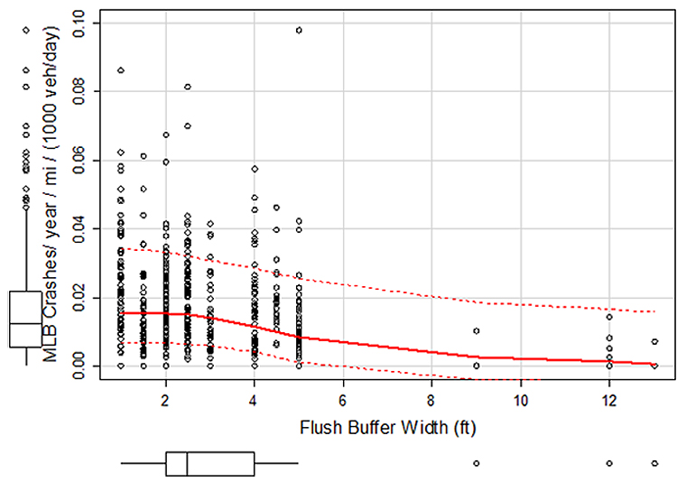
Note: MLB = managed lane or buffer related crashes, mi = mile, veh = vehicle, ft = feet. Figure 14. Chart. California, managed lane and buffer crashes by buffer width. Figure 14 graphs the managed lane and buffer crash rate. To also consider the crashes on general-purpose freeway lanes, Figure 15 (California) and Figure 16 (Texas) were created. Figure 15 illustrates the per lane crash rate for all freeway crashes within the California dataset. Like the findings for managed lane crashes (shown in Figure 14), the per lane crash rates are similar for buffers less than 3 ft. For buffer widths of 4 ft and greater, the trend shows lower crash rates. The data for flush buffers in Texas (see Figure 16) show a similar trend of higher crash rates for the more narrow buffers (defined in this dataset as being 2 ft and less) as compared to wider buffers (5 ft, for the Texas dataset). Figure 16 also shows the trend for sites with pylons. When pylons are used, the buffer width is always 4 ft or more. The trend line indicates that pylons used with 6-ft buffers have fewer freeway crashes per lane; however, few sites had the 6 ft buffer. Additional sites are needed to form a strong conclusion regarding the relationship between crashes and the width of buffers with pylons. In addition, the crash dataset used for this analysis included all freeway lanes. Preference would be to use a dataset that only includes crashes on the lanes on either side of the pylons. Given that the Texas crash dataset does not identify the lane for the crash, a research study that uses a crash narrative-review approach would be needed. The data in Figure 16 do show a higher crash rate for sites with pylons in the buffer as compared to sites with a 5-ft flush buffer. This relationship was found to be statistically significant (see Table 18). 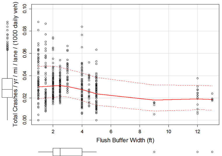
Note: yr = year, mi = mile, veh = vehicle, ft = feet. Figure 15. Chart. California, freeway crashes by buffer width. 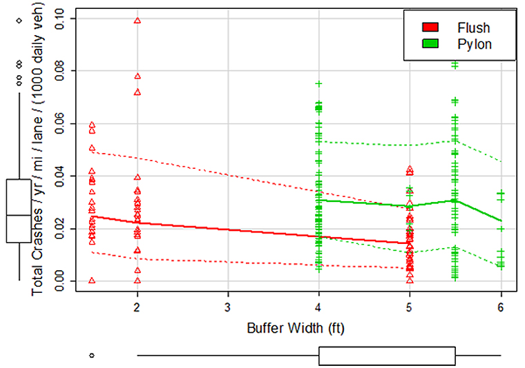
Note: yr = year, mi = mile, veh = vehicle, ft = feet. Figure 16. Chart. Texas, freeway crashes by buffer width and presence of pylons (triangles for flush buffers without pylons and dashes for buffers with pylons). | |||||||||||||||||||||||||||||||||||||||||||||||||||||||||||||||||||||||||||||||||||||||||||||||||||||||||||||||||||||||||||||||||||||||||||||||||||||||||||||||||||||||||||||||||||||||||||||||||||||||||||||||||||||||||||||||||||||||||||||||||||||||||||||||||||||||||||||||||||||||||||||||||||||||||||||||||||||||||||||||||||||||||||||||||||||||||||||||||||||||||||||||||||||||||||||||||||||||||||||||||||||||||||||||||||||||||||||||||||||||||||||
|
United States Department of Transportation - Federal Highway Administration |
||
 = Number of crashes at one analysis period at the ith site.
 = An actual count of crashes for the jth analysis period at the ith site, such that
  .
. = Poisson distribution parameter at the ith site.
 for the Poisson distribution.
 , a model can be developed as shown in
  has units of crashes/mi-yr.
 = Fixed exponent.
 = Vector of fixed effects (i.e., explanatory variables).
 = Vector of fixed-effects coefficients.
 = Random effect for ith site.
 = is the expected yearly crashes per mile, given AADT and the variables represented in X.
 and
and  from the site random effects variability alongside the coefficients for the fixed effects (i.e.,
  and
and  ). The quantity represents the expected number of crashes per amount of exposure at any site. The next section reviews results from estimating the model from the methodology just described.