Freight Performance Measure Approaches for Bottlenecks, Arterials, and Linking Volumes to Congestion Report
Chapter 3. Measuring Signalized Arterial Congestion
3.1 Introduction
Unlike freeways where there has been a fair amount of analysis activity, measuring signalized arterial performance has been elusive. Historically, agencies have had the luxury of intensive roadway data collection systems on freeways with which to track speeds and volumes at a specific point. These are useful on freeways because of uninterrupted flow and can be used for a variety of control strategies. These data, which would have to be collected mid-block on a signalized arterial, are not useful for signal control—what matters are conditions at the signal itself. However, vehicle probe and roadway-based travel-time collection systems (such as Bluetooth and toll tag readers) offer the potential for collecting arterial performance data, but several barriers still exist:
- Sample Size—Especially relevant when trying to measure reliability, which is based on the variability in travel times. Are there sufficient numbers of trucks to allow dependable performance metrics to be computed?
- Truck Speeds—Are the speeds of trucks representative of the traffic stream as a whole? Do they match well under certain flow conditions and not others? Can adjustment factors be developed?
- Truck Operations—Truck travel patterns can be significantly different from passenger cars which are usually studied in congestion analyses. For example, truck deliveries are concentrated during weekday mid-day periods, which are not usually studied in congestion analyses.
- Free-Flow Speed (or Reference Speed)—The determination of free-flow or reference speed on arterials, which determines when delay is being measured, is far from settled. (Here we use the term “reference speed” to avoid confusion because free-flow speed may have a strict definition, as in the Highway Capacity Manual (HCM).) Several approaches have been taken, including: examining speeds during off-peak hours (possible with continuously collected data); based on speed limit; and based on physical setting and “class” of roadway. Depending on what approach is taken, delay computation will vary significantly.
- Arterial Performance Measures—Many agencies have developed arterial performance measures, but a large number of measures are used to gauge signal performance rather than how users experience travel time over a section. They are primarily used as diagnostics for identifying problems with signal operations (e.g., phasing, progression). Some of these measures include queue length, failed cycles, and stopped time. These measures are understandable because they help agencies manage their system, but they are a level below hereunder-based performance, which is to measure the experience of travelers. Therefore, most, if not all, of the travel time-based measures used for freeways are appropriate for arterials as well. There may be additional ones worth considering, for example, number of stops along a signalized section resonates with travelers as a meaningful measure.
In the broader realm of arterial performance management, it is desirable to construct a fully integrated set of performance measures, where higher-level performance measures (outcomes) are directly influenced by changes in lower-level measures. In the general literature on performance measurement, this is described as a program logic model. (Bureau of Justice Assistance.) Figure 7 shows how this model can be adapted for arterial performance management. The distinction between “outputs” and “outcomes” is that outcomes are experienced directly be the user, while outputs are related to how signals perform (which in turn influence outcomes). Note that measures related to daily operations activities feed into a broader context, which indicates a community’s overall vision and goals. In addition, as one goes higher in the structure, the influence of other factors outside of arterial performance enters the picture.
The Guide addresses these issues in the subsequent parts of this section.
Figure 7. Flow chart. Program logic model adapted for arterial performance management.
(Source: Cambridge Systematics, Inc.)
3.2 Data Sources for Monitoring Signalized Arterial Performance
3.2.1 Travel-Time Data
Measuring arterial travel time is challenging. Since the movement of vehicles is interrupted by signals, estimates based on average speeds from loop detectors or radar (typically placed mid-block) are inaccurate. Past approaches to arterial travel time estimation have been synthetic: Models have been used with available data to derive—rather than to measure directly—arterial travel time. (Kwong, K. et al., A Practical Scheme for Arterial Travel Time Estimation Based on Vehicle Re-Identification Using Wireless Sensors, Transportation Research Board 89th Annual Meeting, January 11 to 15, 2009, Washington, D.C.) The data used by these procedures includes the volumes and speeds from mid-block detectors and sometimes information on signal phasing, but traffic flow models of some sort also are used to derive travel time.
All of the data sources covered in section 2.1.1 are useful in signalized environments, with the following caveats and additions.
3.2.1.1 ITS Roadway Detectors
Equipment that detects volume, speeds, and lane occupancy are of limited use on arterials where they are placed at mid-block locations; they are sometimes referred to as “system detectors.” As discussed above, mid-block speeds cannot be used to derive arterial travel times because most of the delay occurs on intersection approaches.
3.2.1.2 Vehicle Signature Reidentification
This data source uses sensors that measure changes in Earth’s magnetic field induced by a vehicle, and processes the measurements to detect a vehicle. Each vehicle is defined by its own unique signature. Matching individual vehicle signatures from wireless magnetic sensors placed at the two ends of a link produced travel times. (Kwong, K et al., Arterial Performance Measurement with Wireless Magnetic Sensors, American Society of Civil Engineers, 2011.)
3.2.1.3 Traffic Signal Control Data
In addition to using system (mid-block) detectors coupled with modeling, several researchers have developed procedures for estimating travel time from signal control data. These data are “event-based” as they relate to either the presence or absence of a vehicle at a point on or near the signal approach, or the status of the signal phasing. Liu et al. devised a “virtual probe” simulation using both vehicle-actuation and signal phase change data in a synchronized manner. (Liu, H. X., W. Ma, X. Wu, and H. Hu, Development of a Real-Time Arterial Performance Monitoring System Using Traffic Data Available from Existing Signal Systems, prepared for Minnesota Department of Transportation, December 2008.) These data are time-stamped allowing the reconstruction of the history of traffic signal events along the arterial street. In the simulation, the virtual probe vehicle’s trajectory is traced in time and space, and its status at any point in time is dependent on the underlying data. When the vehicle “completes” its trip, total travel time is recorded. In the absence of directly measured travel times and delays, this approach would work for measuring arterial performance at the level relevant for freight bottleneck analysis, assuming that the detailed signal event data are available and the virtual probe procedures has been calibrated and is available as user-grade software. Liu et al. also developed a method for estimating queue length based on shock wave analysis.
Day et al. recently extended this approach of using high-resolution controller event data. (Day, C. M., E. J. Smaglik, D. M. Bullock, and J. R. Sturdevant. Real-Time Arterial Traffic Signal Performance Measures. Publication FHWA/IN/JTRP-2008/09. Joint Transportation Research Program, Indiana Department of Transportation and Purdue University, West Lafayette, Indiana, 2008. DOI: 10.5703/1288284313439.) They developed a portfolio of performance measures for system maintenance and asset management; signal operations; non-vehicle modes, including pedestrians; and travel time-based performance measures for assessing arterial performance. Most of these measures relate to evaluating how well signal timing (progression) and phasing are performing and can indicate specific areas where improvement is needed. Liu reinforces this observation: (Liu, H. X., Automatic Generation of Traffic Signal Timing Plan, Research Project. Final Report 2014-38, September 2014.)
“Classical measures of effectiveness (MOE) for signal coordination include travel time, vehicle stops, arrival type, arrivals on green (AOG), percent arrivals on green (POG), and bandwidth. Although arterial travel time and vehicle stops are intuitive to drivers, AOG, POG and bandwidth are more useful from traffic operation perspective.”
So, as shown back in figure 7, different levels of performance measures exist. For the purpose of freight bottlenecks analysis, travel time-based user perspective measures are the most appropriate. Adding the signal event-based measures would be a good addition if such a system already was in pace. For a State DOT, this means having access to every signal controller in the State, at least for higher order highways.
While the focus of this detailed “event-based” work is clearly on the signal operation and maintenance, several aspects are of interest to measuring arterial corridor performance.
First, the discussion of signal progression measures is relevant. They introduce the concept of delay at individual signals, including its components. In addition to deriving delay from models such as the Webster and HCM equations, Day et al. also observe that:
“… at locations where the arrival profiles can be directly measured, it is possible to analyze the delay by calculating the area between the arrival and departure curves. This is done by directly considering the cumulative arrivals and departures over time based on vehicle detections and phase status. The departure curve can be measured either directly using departing vehicle counts or by assuming a departure profile based upon the actual green times.”
Second, Day et al. present methods for calculating arterial travel time based on previous work by Remias et al. (Remias, S. M., A. M. Hainen, C. M. Day; T. M. Brennan, Jr., H. Li, E. Rivera-Hernandez, J. R. Sturdevant, S. E. Young, and D. M. Bullock, Performance Characterization of Arterial Traffic Flow with Probe Vehicle Data, Transportation Research Record No. 2380, Transportation Research Board of the National Academies, Washington, D.C., 2013. DOI: 10.3141/2380-02.) They discuss five data collection methods discussed in chapter 2 but have named them differently. All of these produce estimates of travel time along some distance of the arterial:
- Agency-driven probe vehicles.
- Vehicle reidentification using pavement sensors.
- Vehicle reidentification using MAC address matching (Bluetooth).
- Crowd-sourced data (commercially available vehicle probe data).
- Virtual probe model (using high-resolution event data at each intersection along an arterial to estimate probable vehicle trajectories along the corridor).
They also present three methods for reducing the data. This assumes that travel times are available for multiple short segments within the span of an arterial corridor. Ideally, the segments are defined by signal location:
- Origin-Based—Data are summarized for increasing segment groupings starting at the origin. If the origin is point A and successive intersections are labeled as B on up to F (the destination), the segmentation is: A-B, A-C, A-D, A-E, and A-F.
- Destination-Based—Here the destination is the “anchor point,” so the segmentation is: A-F, B-F, C-F, D-F, and E-F.
- Individual Segments—Here the segmentation is A-B, B-C, C-D, D-E, and E-F. This reduction method allows the calculation of control delay, where control delay is the travel time minus the time required to proceed through the segment at the free-flow speed. (They used the fifth percentile travel time to define the free-flow speed.)
3.2.1.4 Crowd-Sourced (Commercial Vehicle Probe) Data
Overview: Signalized arterial roadways function with far more speed variability than limited access highways, particularly those highways operating at free-flow speeds. Under normal conditions, the majority of vehicles moving on a limited access highway operate within a relatively tight speed distribution. On signalized arterials, however, it is typical for a vehicle to be moving across a wide range of speeds or to be stopped for significant amounts of time. This key difference between the two road types is demonstrated using samples of the American Transportation Research Institute’s (ATRI) truck GPS data in figures 8 through 11.
Figure 8 illustrates spot speeds along a typical stretch of limited-access highway. For the most part, vehicles operate on this roadway near the speed limit (though many are equipped with speed governors).
Figure 8. Map. Interstate spot speeds.
(Source: American Transportation Research Institute.)
The lack of variability among the spot speed measurements is further demonstrated in figure 9, where more than 80 percent of the measured spot speeds are between 55 and 65 miles per hour.
Figure 9. Graph. Distribution of sample Interstate spot speeds.
(Source: American Transportation Research Institute.)
As figure 10 shows, however, the stop-and-go nature of signalized arterials results in a variety of speeds within a small roadway segment.
Figure 10 Map. Spot speeds along an urban signalized arterial.
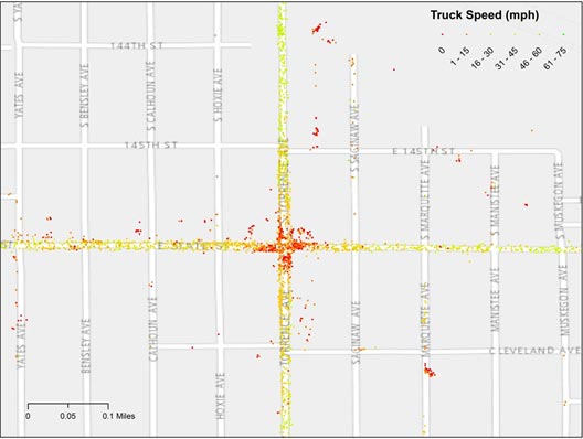
(Source: American Transportation Research Institute.)
This is further demonstrated in figure 11. Nearly 9 percent of measured spot speeds are stopped, while 39 percent are operating in the 25 to 35 miles per hour range.
Figure 11. Graph. Distribution of sample urban signalized arterial spot speeds.
(Source: American Transportation Research Institute.)
Due to these differences, measuring performance on signalized arterials is more complex than measuring performance on limited access highways. Thus, it is likely that enhancements to standard highway measurement methodology are necessary for signalized arterials, including methodologies for identifying bottlenecks.
Approaches: Spot Speed versus Travel Time: There are two basic approaches for calculating average speed/travel times and attributing those measures to roadway segments using vehicle probe data: the spot speed approach and the travel-time approach.
Spot Speed: Spot speed calculations measure clusters of single points on a given roadway segment during a given time period. A single spot speed measurement, represented for instance as a single point in figures 8 or 10, captures the rate of travel a vehicle is moving at a certain latitude/longitude point and at a certain time. For a small stretch of rural Interstate highway (one mile, for instance), a single point may be sufficient to identify free-flow performance over a short time period.
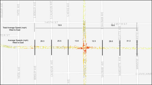
Due to the variability of speeds within short distances, however, arterials must be approached differently. Figure 12 shows average spot speed measurements within the earlier arterial roadway example. The road has been segmented into small sections (approximately 300 feet) to show the variability of average speeds along the roadway, demonstrating that spot speed analysis might not fully capture congestion problems on signalized arterials.
Figure 12. Map. Average spot speed measurements.
(Source: American Transportation Research Institute.)
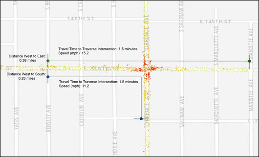
Travel Time: Travel time calculations, on the other hand, focus on point-to-point calculations rather than a single moment in time. Such a calculation can be useful at signals in particular because it has the potential to capture the duration of a stop. Examples of these calculations are illustrated in figure 13.
Figure 13. Map. Travel time measurements along an urban arterial.
(Source: American Transportation Research Institute.)
The downside to this approach, however, is that vehicle probes cannot be compelled to produce a data point at two specific locations in the way a fixed traffic sensor could. Thus, individual point-to-point travel times must be layered upon or attributed to road segments that are crossed. It should also be noted that travel times, such as those in figure 13 are further complicated by direction—for an eastbound vehicle, it may take a different amount of time to turn north, south or maintain direction.
As of this writing, vehicle probe data from commercial sources are only starting to distinguish whether spot speeds or point-to-point travel times were used to calculate the data they provide, which as of now travel times (or speeds) are assigned to directional roadway “links.”
3.2.1.5 Summary of Arterial Data Collection Methods for Travel Time and Delay
Table 6 provides a synopsis of the major types of data collection systems for travel time. All types except for crowd-sourced data require that agencies deploy and maintain field equipment. The ability to measure signal control delay is possible with these sources if the data segmentation coincides with signal location. Estimation of delay using signal event data synthetic, i.e., it relies on models.
(Source: Remias et al.; “virtual probe” assessment added by Cambridge Systematics, Inc.)
The data types identified in table 7 represent those that are available as of the writing of this report. It is possible that vendors currently offering vehicle probe data based on segmentation will soon provide “traces” of individual vehicles that allow constructing travel times between origins and destinations (O/D). These O/D travel times would be directly measured rather than synthesized.
One further note on crowd-sourced (vehicle probe) data. Recent evaluations from the University of Maryland and Virginia Center for Transportation Innovation and Research (VCTIR) suggest that the accuracy of these data is questionable on streets that have very congested, oversaturated conditions (multiple-cycle failures). Accuracy problems also exist on lower-order functional classes, where probe samples are likely to be small. (Considerations and Challenges for Monitoring Arterial Street Performance.) For the purposes of arterial performance monitoring and bottleneck identification, where we are primarily interested in the relative rankings and trend analysis, the accuracy problem is not as severe as for other uses such as traveler information. As vendors gain more experience in collecting and processing travel-time data, the accuracy problem may be reduced, but there is no guarantee of that happening. For example, more direct tracking of vehicles over a facility—rather than relying on instantaneous speed readings—offer promise. For the moment, users need to be aware of the accuracy problems especially when making benefit estimates.
3.3 Recommended Procedure for Measuring Signalized Arterial Congestion
3.3.1 Criteria for Developing the Measurement Procedure
As discussed above, a variety of technologies and methods can be used to calculate signalized arterial performance. The methods include direct measurement of travel time and delay, synthetic (model) derivation of travel time and delay, and a combination of direct measurement and models. The literature covers arterial performance measures extensively, but many of these relate to signal maintenance and operation, and are only indirect indicators of congestion. With that in mind, we establish several criteria that a measurement procedure should meet:
- The user’s perspective, not the facility perspective, should define arterial congestion performance. Travelers experience the whole trip; isolated portions of it influence trip performance but the whole experience is important to travelers. This criterion implies that travel times be the basis for arterial performance measures for congestion. Using travel times also is consistent with freeway performance measurement and travel times resonate with the general public; they are easy to communicate.
- The best way to develop travel times is to measure them directly. Of the technologies listed in table 6, agency probe vehicles and the vehicle reidentification technologies accomplish this. Crowd-sourcing methods may or may not; these currently are used by private vendors who employ proprietary data reduction methods, and it is difficult to know if they develop travel times from tracking individual vehicles over a distance or use instantaneous vehicle speed measurements. If vendors ever develop data based on true time-space traces for individual vehicles, then directly measured travel times will be available.
- Recognizing that the use of agency probe vehicles will result in a limited sample and the deployment of roadway-based reidentification equipment is expensive, the current generation of crowd-sourced data can be used to measure arterial performance.
- Continuously measured travel times produce distributions of travel times. Having access to the complete travel-time distribution allows the calculation of reliability and provides a more complete picture of performance.
- Measure delay at individual signals along an arterial corridor. The ability to identify specific bottlenecks along a corridor is a vital step in performance management. Once the performance of the arterial corridor is established, a “drill-down” capability will identify where problems exist.
3.3.2 Arterial Performance Measures
Travel times establish a wide variety of arterial performance measures. The following section provides the recommended minimum set of performance measures. Both corridor-wide and signal-based measures are included.
3.3.2.1 Corridor-Wide Travel-Time Data Reduction
The first step in developing corridor-wide measures is to work out the segmentation of the corridor so that the data can be properly reduced. Because of issues of “time-distance displacement” in combining data, the corridor should not be excessively long: 10 miles is a reasonable maximum. (Note: If travel times from multiple links are added to get the route travel time for a given time period, this will not correspond to the travel time measured from a vehicle’s perspective, which will pass over downstream links at different times.) Above that, care must be used in interpreting the results.
In all likelihood, the corridor of interest will be longer than the data collection segments that comprise it. Therefore, a method for combining the measurements for the data collection segments (e.g., where a reidentification detector is located or the links on which crowd-sourced travel times are reported) into the corridor is needed. Four methods can be used:
- The most direct method is simply to track the travel times of individual vehicles throughout the length of the entire corridor and develop the travel-time distribution from them. This currently is only possible with the reidentification technologies. It is the “purest” of the methods as the corridor travel time is directly measured. However, there are problems with this approach.
- Sample sizes may be small, because of vehicles entering and leaving the corridor at different points.
- Due to the possibility of travelers making intermediate stops at activities along the corridor, some recorded travel times will be excessively long. Statistical procedures have been developed to weed out these long trips, but they are post hoc in nature and may result in excluding sound data. (For example: Salek Moghaddam, Soroush and Bruce Hellinga, Evaluating the Performance of Algorithms for the Detection of Travel Time Outliers, Transportation Research Record No. 2338, Washington, D.C., 2013.)
Keeping the corridors reasonably short in length, minimizes problems, even for lengths shorter than the 10 miles recommended above.
- Using crowd-sourced (e.g., vendor-supplied travel-time data), develop travel-time distributions for each data collection segment first, and then combine to get the corridor distribution. (Note: It is assumed that vendor-supplied travel-time data are available for short highway segments such as Traffic Message Channel segments.) The moments of the distributions for the individual data collection segments are calculated. These include the following metrics for both travel time and space mean speed: minimum and maximum values; 1st, 5th, 10th, 15th, 20th, 25th, 30th, 40th, 50th, 60th, 70th, 75th, 85th, 90th, 95th, and 99th percentiles; mean; and variance. Corridor metrics are simply the sum of the data collection segment metrics. Past research has found that travel times on adjacent links are not statistically independent (i.e., they are assumed to be correlated), and hence variances and percentiles cannot be added (but means can). (Mahmassani, Hani et al., Incorporating Reliability Performance Measures into Operations and Planning Modeling Tools, Report S2-L04-RR-1, Transportation Research Board, 2014.) Recent work by Isukapati et al. suggests that in practice, they can be additive. (Isukapati, Isaac Kumar, George F. List, Billy M. Williams, and Alan F. Karr, Synthesizing Route Travel-Time Distributions from Segment Travel-Time Distributions, Transportation Research Record No. 2396, Transportation Research Board of the National Academies, Washington, D.C., 2013, pp. 71–81. DOI: 10.3141/2396-09.) However, their work is based on examining a single freeway corridor with relatively uncongested conditions—the applicability to congested and/or arterial conditions is unknown.
- Using crowd-sourced (e.g., vendor-supplied) travel-time data, develop corridor-wide travel times first, and then create the corridor distribution from them. In this approach, a corridor travel time for each time epoch (e.g., every five minutes) is created. These travel times are then the observations in the travel-time distribution from which congestion and reliability metrics are created. This method avoids any thorny statistical problems with combining distributions and most closely resembles data collected from direct observation of travel times from end to end.
- Apply the virtual probe or trajectory method to crowd-sourced data. This is not a distinct method but an extension to method 3 above, which has the problem of not precisely replicating the passage of vehicles over the facility in time and space. (Method 2 also suffers from this time-distance displacement but there is no easy way to address it for percentiles; mean values could be used, however.) (SHRP 2 Project L02 developed a Monte Carlo simulation approach to this problem but it is cumbersome to implement. See: List, George L. et al., Guide to Establishing Monitoring Programs for Travel Time Reliability, Report S2-LO2-RR-2, Transportation Research Board, 2014.) This is less of a problem for relatively short facilities, such as the recommended 10 miles. However, as trip lengths extend, the problem becomes exacerbated.
Recommendations: Recommendations based on this assessment of arterial travel-time data reduction are:
- Using the principle that the best way to develop travel times is to directly measure them, method 1 should be the preferred method, but it has limitations for arterials because of small sample sizes and interrupted trips. It also is applicable only to the reidentification data collection technologies. Therefore, the preferred approach is method 4, especially for long corridors. Method 3 will suffice for corridors that are not longer than 10 miles.
- Adding segment distributions to obtain percentiles, which are the basis for most reliability metrics, is not recommended for facility performance. Serious theoretical questions exist that have not been adequately addressed with empirical evidence, and we see no simple way of accounting for the time-distance displacement problem with this method. Additional research may override this recommendation or develop adjustments for its application.
- If only mean travel times are desired, and then adding mean segment travel times to obtain facility travel-time is acceptable.
3.3.2.2 Treating Missing Data in the Calculations
For all of the above methods, the analyst will most likely have to deal with missing data. Because the foundation of performance measurement is to create an overall travel time for a facility as the sum of the travel times on shorter segments, missing data can influence the outcome. For example, suppose method 2 is being used. There are four short segments whose travel times need to be summed. For a given five-minute time interval, only three of the segments have travel times present.
The first step in deciding what to do is to assess the data for the occurrence of missing data for the time periods being analyzed. This analysis will provide the analyst with information on what to do next. Then, three strategies can be used to account for the missing data:
- Discard the time interval if less than 100 percent of all segment travel times are present. The analyst may decide that the travel times on each segment are so unique that any factoring or imputation method will produce misleading results. This strategy will be adequate if there are not too many time intervals that are discarded.
- Impute values for the missing segment travel times. Imputation creates new values based on the typical patterns of a segment. For example, the average travel time for the same time period for the same day of week may be used. A more detailed look at imputation can be sound in the SHRP 2 L02 Guidebook. (Establishing Monitoring Programs for Travel Time Reliability.) However, using overall averages cannot account for the variations in travel times caused by disruptions that may occur on a given day, so using imputation is a judgment call for the analyst.
- Treat the existing segment travel times as a sample and expand it based on length. In this approach, the sum of the travel times for the segments with travel times is expanded based on the ratio of the facility length to sum of the lengths for the segments with travel times. As with imputation, this approach has limitations—it assumes that conditions on the segments with travel times are representative of the missing segments. If this approach is used, a minimum length for the existing segments should be established—below this threshold the data cannot be expanded. It is recommended that at least 50 percent of the facility length be present.
3.3.2.3 Signalized Arterial Performance Measures
Individual Intersections: Many performance measures have been identified for signalized intersections but most of them are to help maintain and operate signals, not for performance reporting from the user’s perspective. For the purpose of the user-based performance reporting, signal control delay (the actual vehicle-hours minus the vehicle-hours that would be experienced to proceed through the segment at the reference speed) is the most useful measure. This is computed only for the shortest segment in the data that has a signal at the downstream end. Reference speed is defined in the next subsection.
Signalized Arterial Performance Measures: Segment and Corridor: The following measures for congestion and reliability are recommended:
- Total Delay (Vehicle-Hours and Person-Hours)—Actual vehicle-hours (or person-hours) experienced in the highway section minus the vehicle-hours (or person-hours) that would be experienced at the reference speed.
- Mean Travel-Time Index (MTTI)—The mean travel time over the highway section divided by the travel time that would occur at the reference speed.
- Planning-Time Index (PTI)—The 95th percentile Travel-Time Index computed as the 95th percentile travel time divided by the travel time that would occur at the reference speed.
- 80th Percentile Travel-Time Index (P80TTI)—The 80th percentile Travel-Time Index computed as the 80th percentile travel time divided by the travel time that would occur at the reference speed.
3.3.2.4 Calculating the Reference Speed
Discussion: As noted above, performance measures require a baseline or benchmark from which to calculate them; this is based on a fixed reference speed predetermined by the user. In the literature, the free-flow speed is often used as the reference speed, but some agencies may want to use an alternative reference speed. The purpose of the reference speed is to determine the point at which “congestion” begins.
The biggest issue faced on signalized arterials is whether or not the presence of signals should be accounted for in establishing reference speed. Under very light traffic conditions, some delay will occur at signals in order to address side street demand. On the other hand, to assume that signals do not exist (i.e., using mid-block speeds as a basis) implies that signals on the arterial are perpetually green. The issue is to decide which of these cases is closest to ideal conditions.
Several methods exist for computing the reference speed:
- Assume a fixed-reference speed value for all facilities of a given type. Using this method a single value for all signalized arterials would be used.
- Base the reference speed on the speed limit. Some applications use the speed limit or a constant adjustment to it; the Florida DOT uses speed limit plus five miles per hour. (Moses, Ren and Mtoi, Enock, Evaluation of Free Flow Speeds on Interrupted Flow Facilities, Final Report, Project No. BDK83 977-18.)
- Base the reference speed on the speed at which maximum throughput volume occurs. Freeway analysis uses this method where it is noted that from the speed-flow curve, the maximum throughput occurs in the 45 to 54 miles per hour range. We are unaware of any application of this concept to signalized arterials as maximum throughput depends on signal timing.
- Use the speed indicative of a certain Level of Service as the reference speed, as calculated by the HCM. For example, Level of Service C occurs when signalized arterial speeds are 50 to 67 percent of the base free-flow speed. However, the user must select the actual value in the range.
- Use a speed that is indicative of users’ “reasonable expectations.” This approach is based on the observation that users acclimate to prevailing conditions, and where their travel experience is congested, do not expect to travel at the speed limit or free-flow speed. Values related to the mean or median speed are often proposed for the reference speed. A problem with this approach is that user perceptions will vary in urban versus rural areas, and can change for different facilities within an area. Moreover, selecting the reference speed is often done without scientifically determining what user expectations are.
- Use a combination of factors to set the reference speed. In the HCM, a number of factors determine signalized arterial free-flow speed: speed limit, median type, curb presence, access points, and signal spacing.
- Use travel-time data during off-peak hours. With the advent of continuously collected travel-time data, it is now possible to “observe” speeds under light traffic conditions. Approaches here use data from low-volume time periods, such as overnight hours between midnight and 5:00 a.m. or early morning weekend hours. The data are polled and a moment of the distribution is used as the reference speed—the 85th percentile is common. Three problems exist with this empirical approach. First, while this is a reasonable approach for freeways, signal timing during the off-peak periods may be biased toward providing green time on the mainline arterial. Second, even with freeways, if data are used periodically (e.g., every year) to update the reference speed, a constant base no longer exists, and performance trends may the result of a changing reference speed as opposed to changes in congestion level. This problem is remedied by selecting a permanent reference speed based on data.
The third problem with using field data is that there appears to be a significant difference in the free-flow speeds of passenger cars versus trucks. Data from the 2014 NPMRDS, which distinguishes the speeds of passenger cars and trucks, were analyzed for Florida and Tennessee. Free-flow (reference) speeds were computed separately for passenger cars and trucks for TMCs individually. The results are shown in table 7. The overall speed differences are dramatic: truck reference speeds on Interstates on 7.8 miles per hour lower for Tennessee and 9.6 miles per hour lower for Florida. The difference is about one-half that for non-Interstates. A closer look revealed that most truck reference speeds never get much above 65 miles per hour, probably due to speed governors and/or company driving policies.
(Source: Cambridge Systematics, Inc.)
The truck/passenger car speed differential, at least where the current NPMRDS is concerned, raises the issue of what speed measurement to use to establish reference speed. If the passenger car speeds are used, trucks will automatically be assigned some delay, even they are traveling at “their” reference speed. Using truck-only speeds would be one way to set the overall reference speed, but the number of trucks reporting speeds in any given epoch may be very low, or non-existent, especially on lower order highways. Some probe databases also do not report truck-only speeds. Finally, even under low-volume conditions, truck reference speeds could be low due to geometric conditions such as bad grades and curves. Setting the overall reference speed equal to truck reference speed would mean that these locations don’t register as bottlenecks, given the way that performance measures are calculated.
A test was conducted to determine what effect different reference speed thresholds have on results. ITS detector data were used for nine highway sections in Atlanta for 2010; these have the advantage of direct volume measurements paired with speed measurements (table 8). Four thresholds were considered: the section’s free-flow speed, maximum throughput speed (52 mph, based on the HCM’s speed-flow curve for freeways), 40 mph, and the section’s median speed. Free-flow speeds were in a narrow range from 67 to 71 mph, but the median speeds varied greatly, from 31 to 66 mph, indicating that travel peaks by direction. Further, median speeds were significantly different for the AM and PM peaks for the same section. Except for delay based on median speed, delay values decreased with decreasing reference speed.
(Source: Cambridge Systematics, Inc.)
For the purpose of ranking bottlenecks, any of the reference speeds, except for the median-based approach, will produce the same ranking of bottleneck locations, though the delay values will be different. If delay based on median speed is included, the ranking order is slightly different, but very close to that produced by the others. Therefore, for bottleneck analysis, we conclude that very little difference in ranking occurs due to the choice of reference speed. Although the analysis was conducted with freeway data, we expect the same pattern to hold for signalized arterials.
One other problem with using a reference speed based on median speed should be noted. The value will change over time, providing an unstable base for tracking annual trends. While it could be held fixed over time, it will tend downward in years when work zones are present, extreme weather occurs, and/or demand is unusually high. It is not clear if users’ expectations are in line with degraded reference speed.
Recommendation: For congestion performance monitoring, the key outcome is the ability to track changes over time—“are things better or worse?” If that is the case, any of the above strategies are reasonable if they are held constant over time. Reiterating one of our principles for performance measures—the best way to develop travel times is to measure them directly—we prefer the data (empirical approach) for arterials. The other methods use surrogates for estimating what travelers experience. The empirical approach assumes that an adequate amount of travel-time data exists for the off-peak time period chosen, which can be either 2:00 a.m. to 5:00 a.m. on weekdays, 6:00 a.m. to 9:00 a.m. on weekends, or both. The 85th percentile should be used as the reference speed from the distribution of speeds for the selected time period. Reference speed should be computed for each of the segments on the facility individually. The reference travel time is then computed as the segment length divided by the 85th percentile speed, and the facility reference travel time is the sum of the individual segment reference travel times. Note that the 15th percentile travel time is equivalent to the travel time that occurs at the 85th percentile speed on a segment. This procedure assumes that a small amount of delay will be built into the reference speed due to signal operation, but under low traffic volumes.
The speed measurements that should be used in reference speed calculation that should be used are for all vehicles combined. This recommendation recognizes that as of this writing, some probe data bases only report this value. In the future, if speeds by vehicle type are universally reported and if reliable vehicle volume data are available, it would make sense to compute reference speeds separately for several categories of vehicle type, and subsequently to compute performance measures for each category. At this time, such a step is over-complicated and stretches the credibility of the existing data.
If sufficient measured speed data are not present, then the speed limit plus five miles per hour should be used. This should provide a reasonable approximation to field data-derived reference speed.
Users should indicate which method they have used in their documentation. Because some agencies already may have policies dictating how reference speed should be calculated, the intent here is to provide a de facto standard so that studies can be compared on an equal basis. Thus, where reference speed policies differ from those recommended here, agencies should compute two sets of performance measures. Their decisions will be driven by the ones based on their policies but the “standard” set will allow others to compare to their work.
3.3.2.5 Calculation Procedures for Arterial Performance Measures
Note: The methods described below can be applied to any highway type for which travel-time and volume data are available for individual segments, such as vehicle probe data. Therefore, they can be used in chapter 4 for the computation of performance measures for any type of freight bottleneck.
The following procedures are specified for two conditions: 1) traffic volumes have been merged into the data using procedures in chapter 2; and 2) no traffic volumes are available. It is highly recommended that traffic volumes be used in order to compute total delay and to weight aggregations properly.
The procedure assumes that in order to compute facility measures, segment measures must first be created.
If travel times are available separately for passenger cars and trucks, then the procedures are used to produce measures for passenger cars, trucks, and all vehicles.
3.3.2.6 Arterial Segments
Reidentification field equipment or by private vendors define location of the segments (e.g., traffic message channels or TMC).
No Volume Data Available
- If travel times are not present in the data, compute them from segment speed and distance for each epoch:
Figure 14. Equation. TravelTime subscript Segment.

Where:
TravelTimeSegment = the travel time for the segment, minutes;
LengthSegment is in miles; and
SpeedSegment is in miles per hour.
- Compute reference travel time:
Figure 15. Equation. RefTravelTime subscript Segment.
Where:
RefTravelTimeSegment = the reference travel time for the segment, minutes; and
RefSpeedSegment = the reference speed, in miles per hour (section 3.3.2.3).
- Compute unit delay for each epoch:
Figure 16. Equation. UnitDelay subscript Segment.

Where:
UnitDelaySegment is delay per vehicle, minutes. If UnitDelay is negative it should be set to zero.
- Create travel-time distribution for the time period of interest (e.g., 6:00 to 9:00 a.m.). Each observation should represent an epoch contained in the time period. Identify the mean, 80th percentile, and 95th percentile (plus any other statistics that are useful for individual cases).
- Calculate recommended performance measures for the time period of interest:
Figure 17. Equation. MTTI subscript Segment.
Figure 18. Equation. PTI subscript Segment.
Figure 19. Equation. P80TTI subscript Segment.
Figure 20. Equation. UnitDelay subscript Segment.
Where:
Subscript e refers to an individual epoch.
Volume Data Available
- Repeat steps 1 and 2 immediately above.
- Compute Vehicle-miles Traveled (VMT), Vehicle-Hours of Travel (VHT), and total delay (in vehicle-hours) for each epoch.
Figure 21. Equation. VMT subscript Segment.

Figure 22. Equation. VHT subscript Segment.

Figure 23. Equation. TotalDelay subscript Segment.

- Create travel-time distribution for time period of interest, using VMT as the weight on each observation. That is, the travel times in an epoch are assumed to be the average of all vehicles traveling over that segment in an epoch. Identify the mean, 80th percentile, and 95th percentile (plus any other statistics that are useful for individual cases).
- Repeat step 4 immediately above using the weighted travel-time distribution; the reference travel time is the same. Total delay is computed in the same manner as unit delay, i.e., the sum of the delay in the epochs in the time period of interest.
3.3.2.7 Arterial Facilities
No Volume Data Available
- Create a dataset for travel times over the facility for each epoch by either: 1) using the vehicle trajectory method (discussed previously); or 2) summing the segment travel times.
- Compute the reference travel time for the facility (RefTravelTimeFacility) as the sum of the segment reference travel times.
- Compute unit delay for the facility for each epoch as the sum of UnitDelay for all segments on the facility for the time period of interest.
- Create travel-time distribution for time period of interest for the entire facility using the data created in step 1. Each observation should represent an epoch contained in the time period. Identify the mean, 80th percentile, and 95th percentile (plus any other statistics that are useful for individual cases).
- Calculate recommended performance measures for the time period of interest:
Figure 24. Equation. MTTI subscript (Facility).
Figure 25. Equation. PTI subscript Facility.
Figure 26. Equation. P80TTI subscript Facility.
Figure 27. TotalDelay subscript Facility.
Volume Data Available
- Repeat steps 1 and 2 immediately above.
- Compute total delay for the facility for each epoch as the sum of total delay for all segments on the facility for the time period of interest.
- Create travel-time distribution for time period of interest for the entire facility using the data created in step 1. The weight on each observation is provided by VMT. That is, the travel times in an epoch are assumed to be the average of all vehicles traveling over that segment in an epoch. Identify the mean, 80th percentile, and 95th percentile (plus any other statistics that are useful for individual cases).
- Repeat step 5 immediately above using the weighted travel-time distribution; the reference travel time is the same. Total delay is computed in the same manner as unit delay, i.e., the sum of the delay in the epochs in the time period of interest.
Cumulative Travel-Time Distribution Function for Arterial Facilities: In addition to the individual metrics computed above, a curative distribution function of the travel times is useful diagnostic purposes. Figure 28 shows an example of this type of plot. This is easily constructed from the travel-time distribution that is specified in the above procedures.
Figure 28. Graph. Example cumulative frequency distribution for travel times.
(Source: Cambridge Systematics, Inc.)
3.3.2.8 Example: Calculating Arterial Performance Measures with the NPMRDS
For this example, we chose U.S. 70, a signalized suburban arterial in Knoxville, Tennessee. It has a basic four-lane cross section with AADTs in the range of 25,000 to 30,000 vehicles per day and an overall signal density of roughly one signal every 0.4 miles. The 2014 NPMRDS was used as the source of travel times. Traffic volumes at the five-minute level are assumed not to exist for this example. The arterial section (facility) selected is the eastbound direction; it is 12 miles long and is comprised of 11 segments (TMCs, in this case). The weekday PM peak period (4:00 to 6:00 p.m.) was selected for analysis. The analysis was conducted for all vehicles, but a similar procedure can be followed if truck-only travel times are desired.
A review of the data revealed two major issues:
- About 3.0 percent of the data had speeds less than 3 miles per hour, and less than 0.2 percent had speeds higher than 55 miles per hour. Many researchers have noticed that the NPMRDS data through 2014 contains travel times that result in both low- and high-speed values. As a result, data less than 3 miles per hour or greater than 55 miles per hour were excluded from the analysis.
- The data completeness for the peak period was 31 percent. That is, only 31 percent of the possible five-minute epochs (time intervals) for the 11 TMCs had data reported.
The reference speed and performance measures for the segments appear in table 9. Even though the reference speeds were calculated from the data and include the effect of signal presence, volumes at the times used (weekends from 6:00 to 9:00 a.m.) are low and signals are likely to be mostly green on the arterial segments. This will influence the performance measures significantly. Because of the low completeness rate, the delay values severely underestimate the actual delay. One way to account for the missing data is to treat the measured delay as a sample and expand it with the ratio of the number of possible epochs to the number of epochs present.
(Source: Cambridge Systematics, Inc.)
Because of the low completeness rate, developing a facility travel-time distribution from which to compute facility performance measures is not tenable. Therefore, the recommended procedure presented in the previous section cannot be used unless the missing data are imputed. Instead, method 2 from section 3.3.2.1 is applied (combine the travel-time distributions from the individual segments). The results appear in the bottom row of table 8. We expect completeness rates to increase as data vendors expand their coverage, but for now analysts must understand completeness patterns in their data prior to undertaking analysis.
You may need the Adobe® Reader® to view the PDFs on this page.
previous | next