Freight Performance Measure Approaches for Bottlenecks, Arterials, and Linking Volumes to Congestion Report

Chapter 4. Analysis of Freight Bottlenecks

4.1 Introduction

This chapter provides the details of how to conduct a truck freight bottleneck analysis. It builds on the information in chapters 2 and 3 and makes reference to their procedures. Figure 29 presents an overview of the analysis methodology presented in this chapter. The methodology is built on the basic steps of identifying potential bottlenecks, ranking bottlenecks to obtain candidate locations, and conducting detailed analysis on the candidates to obtain accurate performance characteristics and to identify specific problems causing the bottlenecks.

The methodology is focused on performance in terms of congestion and travel-time reliability, and the second order effects that result from them. The identification, ranking, and detailed analysis are based on congestion and reliability performance. The methodology does not consider safety, which is clearly a major impact area for trucks, because it was considered to be outside the scope of the project. While this is an area where future work is needed, appendix A is offered to provide some general guidance to analysts who wish to consider safety impacts.

The methodology is built on the premise that truck freight bottleneck performance should be measured empirically rather than estimated through the use of models. As will be discussed, models have their place in the methodology for forecasting conditions, but current year performance at individual bottleneck locations will be calculated using field measured data.

Figure 29. Flow chart. Overview of freight bottleneck analysis methodology.

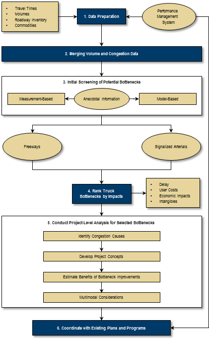
(Source: Cambridge Systematics, Inc.)

4.2 Bottleneck Typology

Before undertaking a freight bottleneck analysis, analysts should be aware of the different types of highway freight bottlenecks that occur. It is useful to categorize bottlenecks into specific types because this aids in the analysis, and indicates which strategies are most appropriate to implement.

For the purpose of this Guide, bottlenecks are broken out into two general types based on the type of delay:

1. Congestion-Based Delay—These bottlenecks are defined by highway congestion, where congestion is caused by several factors. Lower speeds due to traffic flow breakdown define congestion.
2. Non-congestion-Based Delay—These bottlenecks are caused by policies or conditions that cause trucks to deviate from their intended route. Trucks do not necessarily enter congestion, as defined above, and their speeds may be relatively high. However, due to the deviation, truck travel times are increased over what they would have been with the deviation.

4.2.1 Congestion-Based Delay Bottlenecks

4.2.1.1 Geometric-Related Bottlenecks

These bottlenecks are caused by a reduction in roadway capacity, as compared to the prevailing capacity of the highway section. They are related to the physical characteristics of the highway and influence how it operates. Figure 30 shows the types of geometric bottlenecks that occur on freeways. From an operation standpoint, NCHRP Project 03-83 offered the following definition of geometric bottlenecks: (Kittelson Associates et al., Low-Cost Improvements for Recurring Freeway Bottlenecks: Draft Final Report, NCHRP Project 03-83, Transportation Research Board, November 2012.)

Speeds upstream of the bottleneck are less than 30 miles per hour. Speeds at the bottleneck location range between 40 to 60 miles per hour depending of the measurement location (vehicles accelerate as they travel through the bottleneck). Traffic is free-flowing downstream with speeds at or near free-flow speeds (typically above 60 miles per hour). Detector occupancy values are generally above 30 percent upstream and less than 10 percent downstream of the bottleneck location.

Figure 30. Table. Common locations for geometric-related bottlenecks on freeways.

(Source: Recurring Traffic Bottlenecks: A Primer. Focus on Low-Cost Operational Improvements, FHWA-HOP-12-012, April 2012.)

This definition implies that queuing occurs upstream of the bottleneck location (speeds less than 30 miles per hour). It also seems to have been designed for urban conditions only. There clearly will be freeway locations, especially in rural areas, where speeds are higher than 30 miles per hour but less than ideal/free-flow; grades and curves are examples. Because these types of locations are relevant for trucks, this definition is too stringent for this Guide. Therefore, we do not impose any traffic flow restrictions on what constitutes a geometric bottleneck, other than some level of delay is present.

On signalized arterials, the signal itself is a potential bottleneck. Even under light traffic, the presence of the signal will cause some vehicles to stop. However, a definition similar to one above for freeways has not been established.

4.2.1.2 Volume-Related Bottlenecks

Traffic volume (demand) can overwhelm a highway section even if there no geometric restrictions. Examples include:

• Commuter peak period traffic.
• Seasonal vacation traffic.
• Special event traffic.

The distinction between volume- and geometric-related bottlenecks is often blurred. For example, an interchange on-ramp may be poorly designed and would have reduced capacity as a result, while at the same time could add enough volume to the mainline that would cause congestion even if there was no capacity drop. Because they are so intertwined, it is possible to consider geometric and volume bottlenecks as a single class of bottlenecks, but we have considered them separately because it may be helpful in developing bottleneck solutions.

4.2.1.3 Disruption-Related Bottlenecks

Here we use the term “disruption” to mean events that cause a temporary loss of capacity. This type of bottleneck is commonly labeled as “non-recurring” to distinguish them from physical bottlenecks that usually recur with a predictive frequency. Bottlenecks of this type are:

• Incidents.
• Weather.
• Construction/work zones.
• Processing delays.

Examples of processing delays are: border crossings/custom inspections, safety inspections, weighing, and terminal gate processing. With the exception of border crossing/customs, these examples are truck-specific.

4.2.2 Non-congestion-Related Bottlenecks

These bottlenecks are not related to highway operations per se but rather result from policies that delay trucks more than they otherwise would experience without the policy. They may be broken down further into subcategories:

4.2.2.1 Restrictions Requiring Rerouting

• Truck prohibitions and route restrictions.
• Bridge heights clearance issues.
• Truck size and weight limits.
• Hazardous material route restrictions.

4.2.2.2 Restrictions Requiring Changes in Timing of Trip

• Time-of-day restrictions.
• Load restrictions.

4.2.2.3 Restrictions Requiring Other Logistics Changes

• Truck size and weight limits may require lighter loads if no viable alternative routes exist).
• Loading bans.

4.3 Data Required for Freight Bottleneck Analysis

Because this methodology is empirically based, the starting point for bottleneck analysis is travel-time data. Sections 2.0 and 3.0 already have discussed the various forms and provided recommendations. In the ideal situation, the travel-time data has been integrated with traffic volume data (including estimates of trucks) at the lowest spatial and geographic levels of the travel-time data. In the ideal case, the integrated travel-time/volume data is available for the entire area, region, or State being analyzed. If this ideal condition cannot be achieved, the methodology allows for less detailed methods. Other data that are required are:

• Roadway inventory data—These data provide the geometric characteristics of roadways, including cross section (lane width, shoulder width, number, and type of lanes, median width) and the horizontal (curves) and vertical alignment (grades).
• Commodity data—If information on commodities carried by trucks on specific routes is available, it should be assembled. It can be used later in the benefits estimation phase.
• Truck restriction data—Information on where and when truck travel is restricted or banned is required for analyzing some forms of bottlenecks.

These data—especially the travel-time and volume data—already may be present in the agency’s performance management system.

4.4 Bottleneck Performance Measures

4.4.1 Congestion and Reliability Measures

For congestion and reliability, performance measures based on travel time are used. The following measures for congestion and reliability are recommended; these are to be used for all types of highways. Note that the first four measures were recommended as signalized arterial performance measures in section 3.0, which dealt with arterial performance in general. We expand the number of measures here to cover the needs of bottleneck analysis:

• Total Delay (vehicle-hours and person-hours)—Actual vehicle-hours (or person-hours) experienced in the highway section minus the vehicle-hours (or person-hours) that would be experienced at the reference speed. Total delay is only possible to compute if traffic volumes have been integrated. If not, unit delay (delay per vehicle) is substituted.
• Mean Travel-Time Index (MTTI)—The mean travel time over the highway section divided by the travel time that would occur at the reference speed.
• Planning Time Index (PTI)—The 95^th percentile Travel-Time Index computed as the 95^th percentile travel time divided by the travel time that would occur at the reference speed.
• 80^th Percentile Travel-Time Index (P80TTI)—The 80^th percentile Travel-Time Index computed as the 80^th percentile travel time divided by the travel time that would occur at the reference speed.
• Hours of Congestion per Year—Number of hours where vehicle speeds are below the following thresholds:
  • Freeways and Multi-lane highways: 50 miles per hour.
  • Rural Two-Lane Highways: 40 miles per hour.
  • Signalized Arterials: 30 miles per hour.
• 95^th Percentile Queue Length—developed from a distribution of queue lengths, the highway distance where the speeds of contiguous segments upstream of an identified bottleneck location are less than:
  • Freeways, Multi-lane, and Two-Lane Highways—30 miles per hour.
  • Signalized Highways—15 miles per hour.
• Average Queue Length (uninterrupted flow facilities only)—average highway distance where the speeds of contiguous segments upstream of an identified bottleneck location are less than:
  • Freeways, Multi-lane, and Two-Lane Highways—30 miles per hour.
  • Signalized Highways—15 miles per hour.

The reference speed for all highway types should be calculated using the same procedure described in chapter 3 for signalized arterials.

When bottlenecks are intersections or interchanges, it is important to develop performance measure for all approaches into the intersection of interchange. Figure 31 shows why this is necessary. In this case, the actual bottleneck point is a weaving section on the north-south roadway in the interchange. However, because of merging traffic from the east-west roadway, it also influences the performance of that roadway.

Figure 31. Map. Bottleneck at intersection or interchange.

(Source: Cambridge Systematics, Inc.)

4.4.2 Second Order Performance Measures

Second order performance measures are those that emerge as a direct result of changes in congestion and reliability. They are most commonly used to estimate impacts of bottlenecks and the benefits of improving them. The recommended measures are:

• Delay Cost—This is the monetized value of delay. It is computed separately for passenger cars and trucks using the following formulas.

  Figure 32. Equation. Annual passenger vehicle delay cost.

  

  Figure 33. Equation. Annual commercial cost.

  

  Where: the annual vehicle-hours of delay is Total Delay above, broken out by passenger and commercial (trucks).

• Reliability Cost—In addition to the cost of typical delay, studies have shown that highway users also value reliability, or the variability in travel conditions. The valuation of reliability is not nearly as well treated in the literature as that for typical delay. Further, reliability valuation for personal travel has been studied more than for freight travel. One recent study developed a method for computing both typical and reliability portions of congestion costs by using a “travel-time equivalent approach” (SHRP 2 Project C11):

  Figure 34. Equation. TTI subscript e(VT).

  

  Where:

  TTI_e(VT) is the TTI equivalent on the segment, computed separately for passenger cars (personal travel) and trucks (commercial travel);

  TTI₅₀ is the median TTI;

  TTI₈₀ is the 80^th percentileTTI; and

  a is the Reliability Ratio (Value of Reliability (VOR)/Value of Time (VOT).

  • = 0.8 for passenger cars
  • = 1.1 for trucks

The Reliability Ratio (VOR/VOT) of 1.1 suggests that freight interests value reliability slightly more than typical travel time.

However, this topic is still evolving. There is no agreed upon methodology for valuing reliability as of this writing. Users are free to incorporate the value of reliability in their analyses but should clearly document their assumptions. This Guide does not consider reliability costs further.

• Fuel Cost—Is estimated using a simple formula based on fuel efficiency. The following equation may be used separately for passenger vehicles and trucks:

  Figure 35. Equation. Annual commercial cost.

  

  Where: average fuel economy is in gallons per mile (inverse of miles per gallon).

4.5 Initial Screening of Potential Truck Freight Bottlenecks: Geometric- and Volume-Related Bottlenecks

The goal of this step is to obtain a list of potential candidate sites that will be subjected to further analysis.

4.5.1 Screening Based on Performance Data

If travel-time data exist for the entire area of study (e.g., region or State), analysts can perform a scan to identify highway segments where travel speeds are low. The best indication of a bottleneck is when several relatively short (about one mile) contiguous segments have high delay for the same time of day; these should be grouped together. Data should be aggregated to either 5- or 15-minute time intervals for this purpose as these levels will capture the locations that are the most serious problems. If both truck speeds and passenger car speeds are present in the data, then separate scans should be performed for each. Bottleneck locations that coincide are especially worthy of further investigation.

4.5.2 Use of Anecdotal Information

Despite the advances in data that have occurred, local knowledge is still an excellent way to identify congestion problems. Therefore, anecdotal information or the observations of field engineers can be used to verify or dismiss locations identified in the scan and to identify locations the scan may have missed. This can be done through formal or informal surveys of local engineers and planners as well as major shippers and carriers. In conducting the survey, analysts should try to distinguish between “commuter” bottlenecks (weekday peak-period bottlenecks that trucks experience as well) and primary freight bottlenecks (bottlenecks where trucks are the primary users or suffer the most delay).

A preliminary scan can be made on just truck and passenger car speeds. It is recommended that the analyst select multiple time periods for study rather than rely on single average speed value for the entire year. Weekday/non-holiday peak periods are a good starting point as is weekend mid-day (when truck volumes are heaviest). Off-peak periods also should be checked; if low truck speeds are found during both peak and off-peak periods, the likely cause is geometric in nature (e.g., steep grade, sharp curve) or work zone-related.

Table 10 shows an analysis done with NPMRDS data for 2014 for the State of Tennessee. The strategy used here is to compute average truck speeds for weekday peak periods and mid-day as well as for daylight hours on weekends. These four values are then averaged and only highway sections with a speed value less than 45 miles per hour are chosen. The color coding indicates that the sections (TMCs) are contiguous. The length of all the contiguous segments for a route is a good indication of the severity of the bottleneck. Based on small number of locations shown here, the analyst would concentrate first on I-24 southbound in Davidson County. Note that the criteria used here are only one example of those that can be used. Analysts may wish to look at different time periods and change the cutoff speed value for what to consider further.

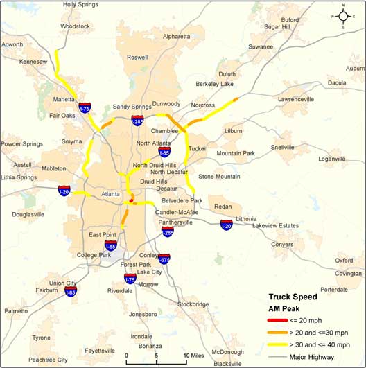
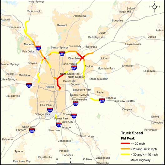
Mapping locations that are caught in the screening process is another useful method for identifying potential bottlenecks for in-depth study. Figures 36 and 37 show truck speeds on Atlanta freeways developed from the NPMRDS for 2014. The roadways experiencing low truck speeds are roughly the same in the morning and afternoon peaks, and mostly correspond to known bottlenecks, primarily freeway-to-freeway interchanges. While the majority of delay is being caused by high passenger car demand and is not specifically truck-related, the total amount of delay to trucks is nonetheless extremely high.

On principal arterials off of the Interstate system, most of the delay is likely due to signals. Figure 38 shows the average truck speeds versus passenger car speeds for weekday daylight hours on signalized principal arterials for two urban counties in Tennessee: Davidson (Nashville) and Knox (Knoxville). For the most part, only small differences exist between the two vehicle types, indicating that the signals are controlling the traffic flow and that no trucks-specific geometric limitations exist.

If travel times have been matched to traffic volumes, then the screening should use either annual total truck delay or unit truck delay as the primary criterion. Assuming that contiguous segments are grouped together, this will give higher weight to locations with multiple “bad” segments.

Table 10. Partial list of potential truck bottleneck locations for Tennessee from National Performance Management Research Data Set scan.

TMC	County	Road Number	TMC Length	Direction	Truck Speeds— Weekday AM	Truck Speeds— Weekday PM	Truck Speeds— Weekday Mid-day	Truck Speeds— Daytime	Truck Speeds— Average
121N11569	Blount	I-140	1.792	Eastbound	42.1	41.0	43.4	50.7	44.3
121P10404	Blount	I-140	1.033	Westbound	43.4	44.8	43.3	42.4	43.5
121P11569	Blount	I-140	0.237	Westbound	29.3	27.7	25.9	26.2	27.3
121N04209	Davidson	I-24	1.198	Southbound	11.8	44.4	30.4	33.9	30.1
121N04222	Davidson	I-24	0.456	Southbound	49.0	20.6	51.8	53.6	43.8
121N04223	Davidson	I-24	0.195	Southbound	52.1	18.1	52.0	53.5	43.9
121N04224	Davidson	I-24	1.159	Southbound	38.5	20.8	45.4	49.4	38.6
121N04225	Davidson	I-24	0.351	Southbound	47.2	21.2	49.8	53.9	43.0
121N04226	Davidson	I-24	0.268	Southbound	49.1	22.1	50.1	53.4	43.7
121N04227	Davidson	I-24	0.262	Southbound	47.9	25.1	48.9	51.5	43.3
121P04175	Davidson	I-24	0.693	Northbound	55.8	20.0	45.5	50.4	42.9
121P04223	Davidson	I-24	0.310	Northbound	19.5	43.8	47.2	47.7	39.6
121P04224	Davidson	I-24	0.730	Northbound	42.8	38.5	45.5	44.6	42.9
121P04229	Davidson	I-24	0.243	Northbound	53.6	20.2	43.4	47.4	41.2
121N04194	Davidson	I-24/I-40	0.372	Eastbound	50.1	22.1	46.8	51.3	42.6
121N04195	Davidson	I-24/I-40	0.149	Eastbound	48.2	16.1	42.2	48.1	38.6
121P04192	Davidson	I-24/I-40	0.085	Westbound	22.2	43.2	47.8	48.1	40.3
121P04194	Davidson	I-24/I-40	0.473	Westbound	28.3	46.4	50.2	52.5	44.4
121P04195	Davidson	I-24/I-40	0.482	Westbound	28.8	42.9	48.0	49.3	42.2
121N04231	Davidson	I-24/I-65	1.040	Southbound	32.8	48.6	47.0	49.5	44.5
121N04232	Davidson	I-24/I-65	0.155	Southbound	20.9	43.2	37.2	40.9	35.5
121P04230	Davidson	I-24/I-65	0.188	Northbound	53.7	20.3	41.2	47.0	40.5
121P04231	Davidson	I-24/I-65	1.019	Northbound	51.9	24.8	40.4	45.7	40.7
121P04232	Davidson	I-24/I-65	0.775	Northbound	48.8	39.5	43.4	45.7	44.4
121N04196	Davidson	I-40	0.526	Westbound	22.7	45.8	51.0	51.2	42.7
121N04206	Davidson	I-40	0.271	Westbound	33.5	44.7	47.9	50.0	44.0
121N04207	Davidson	I-40	0.283	Westbound	25.9	38.3	44.1	47.2	38.9
121N04208	Davidson	I-40	0.226	Westbound	16.7	34.7	44.6	47.1	35.8
121P04205	Davidson	I-40	0.191	Eastbound	50.1	12.5	44.0	48.8	38.9
121P04206	Davidson	I-40	0.245	Eastbound	52.4	17.9	47.3	50.9	42.1
121P04207	Davidson	I-40	0.361	Eastbound	54.6	17.9	50.1	52.7	43.8
121P04208	Davidson	I-40	0.228	Eastbound	54.8	17.1	49.8	53.6	43.8

(Source: Cambridge Systematics, Inc. analysis of NPMRDS data.

Figure 36. Map. Atlanta truck speeds, AM peak.

(Source: Cambridge Systematics, Inc.)

Figure 37. Map. Atlanta truck speeds, PM peak.

(Source: Cambridge Systematics, Inc.)

Figure 38. Graph. Vehicle speeds on primary arterials, Davidson and Knox counties, Tennessee.

(Source: Cambridge Systematics, Inc.)

4.5.3 Model and Inventory-Based Screening

If area-wide data are not available, then the bottleneck scan may be performed with models or roadway inventory data. In urban areas, travel demand forecasting models may be used. The “Full Extent” HPMS data also may be used, as can State-maintained roadway characteristics inventories. What we are looking for here are highway sections that are potential problems based on indicators of congestion rather than direct measurements. Volume-to-capacity (v/c) and AADT-to-capacity (AADT/C) ratio are the recommended indicators. The v/c ratio has a long history in transportation analysis and is based on conditions that exist for a single hour. The AADT/C ratio uses 24-hour traffic (AADT) divided by the two-way capacity. For highly congested locations where multiple hours of the day are congested, the AADT/C ratio captures more of the conditions. Table 11 indicates the AADT values implied by a range of AADT/C ratios.

Table 11. Annual average daily traffic to capacity levels and corresponding annual average daily traffic values.

AADT/C	Freeways (10% Trucks)— Four-Lanes (Ideal Capacity = 2,200 passenger cars per hour per lane (pcphpl)) AADT (Rounded to nearest 1,000)	Freeways (10% Trucks)— Six-Lanes (Ideal Capacity = 2,300 pcphpl) AADT (Rounded to nearest 1,000)	Four-Lane Signalized Arterials (8% Trucks) (Ideal Capacity = 900 pcphpl (based on a saturation flow rate of 1,800 pcphpl and 50 percent green time) AADT (Rounded to nearest 1,000)
9	72,000	113,000	30,000
10	80,000	126,000	33,000
11	88,000	138,000	37,000
12	96,000	151,000	40,000
13	104,000	163,000	43,000
14	112,000	176,000	47,000
15	120,000	188,000	50,000

(Source: Margiotta, Richard; Harry Cohen; and Patrick DeCorla-Souza, Speed and Delay Prediction Models for Planning Applications, paper presented at Sixth National Conference on Transportation Planning for Small and Medium-Sized Communities, Spokane, Washington, 1998.)

The model-based scan is conducted the same way as the data-based scan, except that v/c, AADT/C, and truck AADT as used as the criteria. (These are indicators of the amount of delay.) These measures are computed for every link in the network of interest, paying special attention to the number of contiguous links with high values.

4.5.4 Pulling the Scan Together

The goal of the scan is to come up with a “short list” of bottleneck locations; these are the locations that will be analyzed in more detail and are candidates for improvements. The anecdotal information is reviewed against either the data-based or model-based scans. If possible, the locations should be mapped. Analysts must use their judgment in developing the reduced list of locations. In addition to the technical criteria discussed above, they also should consider:

• Economic Impacts—Does truck delay at a location severely limit the potential for economic growth in a region.
• Connectivity—Is this location a critical link in the truck highway network such as a key bridge or mountain pass?

Once all the factors have been considered, a list of 10 to 50 locations should be identified as the most significant truck bottleneck locations. Bottlenecks should be classified using the guide shown in figure 30.

4.6 Conduct Project-Level Analysis for Selected Bottlenecks: Geometric- and Volume-Related Bottlenecks

4.6.1 Basis for Analysis

The basis for project-level analysis of truck bottlenecks is empirical travel-time data; modeling is not recommended for determining the present state of the bottlenecks. Chapters 2 and 3 present a thorough discussion of travel-time data and its sources. It is assumed that volume data has been merged into travel-time data at the travel time’s lowest levels of spatial and geographic resolution.

4.6.2 Determine the Physical Cause and Initial Range of Influence of the Bottleneck

The first step in project-level analysis is to identify the highway segment on which the bottleneck is located and to determine what geometric and/or volume feature is causing the bottleneck. Once this is established, detailed congestion analysis can proceed. Other than long-term work zones, it is unlikely that the bottlenecks identified during the screening process will be non-recurring in nature. Nearly all—if not all—of them will be recurring bottlenecks that also experience some non-recurring congestion (e.g., incidents, inclement weather, and short-term work zones).

For bottlenecks that primarily occur in urban areas during weekday peak periods, the most common bottleneck types on freeways are interchanges, especially freeway-to-freeway interchanges, and toll facilities. On signalized arterials, intersections especially between two major roadways are commonly the worst bottlenecks, in rural areas, grades, tunnels, and recreational traffic frequently create the worst truck bottlenecks. In rural cases, look for the days of week and times of day when delay is occurring. If most delay occurs during mid-day on most days of the year, the likely cause is a grade or tunnel. If most delay is occurring on or around weekends and holidays, recreational traffic is the likely culprit.

Once the type and location of bottleneck is identified, the initial range of influence is determined. For interchanges and intersections, segments that represent all entering legs of the location are the starting point, even if they were not identified in the scan. That is, the segments that are immediately upstream on the “inbound” direction to the bottleneck should be considered first. Because queues from the bottleneck will form upstream, we then select segments that are upstream from the bottleneck (in the inbound direction) as potential targets for analysis—a starting length of 10 miles is reasonable, it will be adjusted later. Segments on the downstream side also need to be considered because:

• If we ended the analysis at the center of an interchange, we would miss the entrance ramps’ influence on the downstream side.
• Some delay will occur downstream of the last merge area as vehicles come back up to speed after being queued (“getaway” flow).

A distance of 1 mile downstream from the point of the last entrance ramp of an interchange is a reasonable place for the other endpoint of the initial range of influence of the bottleneck. Thus, we have a distance of 11 miles on each inbound route to consider. By studying each of the inbound routes, we also capture spillover effects from the bottleneck. That is, a queue formed by an entrance ramp will not only extend upstream on the mainline but on the ramp and possibly onto the intersecting route as well.

4.6.3 Performance Measure Calculation

The following steps are followed to develop performance measures for the freight bottlenecks.

1. Adjust the Range of Influence—For each of the entry routes into the bottleneck, the range of influence is further refined by determining the range of queuing. Speeds are used as the indicator of queuing. For each epoch in the travel-time data, speeds for each segment in the original range of influence is scanned to determine if queuing is present. The process starts on the segment at the bottleneck location and moves upstream. The idea is to identify a string of contiguous segments that meet the queuing threshold. The thresholds are as follows:
   • Freeways, Multi-lane, and Two-Lane Highways—30 miles per hour.
   • Signalized Highways—15 miles per hour.

   From this analysis, a dataset is created that indicates the queue length for each epoch for each entering route. The queue length is calculated by summing up the segment lengths found to experience queuing.

   Next, for each time period of interest (e.g., weekday AM/PM peaks, weekends), the mean and 95^th percentile queue lengths are calculated. The range of influence is set to the 95^th percentile; this is used in lieu of the maximum queue length because of possible outliers. The segments encompassed by the 95^th percentile queue length are used as the highway distance over which performance measures are computed.

2. Calculate Reference Speed—Chapter 3 presented a method for determining the reference speed for signalized arterials based on analysis of off-peak travel-time data. The same procedure should be used for all other highway types.
3. Calculate Performance Measures for each Bottleneck Entry Route for Each Time Period—Likewise, the chapter 3 method for arterial facilities should be used to develop performance measures related to the bottleneck; these procedures are applicable to all highway types. The 4.5 Conduct Project-Level Analysis for Selected Bottlenecks: Geometric and “facility” in this case is the range of influence previously determined.
4. Rank Bottlenecks by Impacts—For truck bottlenecks, total truck delay is a strong candidate for the ranking criteria. However, as total delay will favor high-volume locations, users may wish to us an alternate criterion such as unit delay, MTTI, PTI, or queue length.
5. Example—I-85/I-285 Interchange, Atlanta, Georgia.
   • NPMRDS data was used to analyze a well-known bottleneck in Atlanta, known locally as “Spaghetti Junction” for its complex ramp pattern (figure 39). Despite being a well-designed system-style interchange, it is still a major source of congestion due to very high (and growing) demand. The NPMRDS data were conflated with HPMS data to obtain AADT values, and the procedure given in chapter 2 was used to decompose AADT into directional 5-minute volumes on each TMC. The results are shown in table 12.

Figure 39. I-285/I-85 interchange, Atlanta, Georgia.

(Source: Cambridge Systematics, Inc.)

Table 12. Performance measures for the inbound legs of the I-85/I-285 interchange, Atlanta, Georgia, 2014.

Leg	Period	MTTI	TTIP80	PTI	VMT	Total Delay (Vehicle-Hours)	Truck Delay (Vehicle-Hours)	Hours of Congestion	95th Percentile Queue Length (miles)
I-285 Northwest	Weekday Mid-day	1.518	1.544	3.557	69,020,721	527,488	57,441
I-285 Northwest	Weekday Peak	2.474	4.033	5.982	79,350,098	1,721,129	170,542
I-285 Northwest	Weekend/Off-Peak	1.267	1.187	1.828	120,538,555	481,309	44,420
I-285 Northwest Subtotal						2,729,926	272,403	1,616	6.0
I-285 Southeast	Weekday Mid-day	1.239	1.195	1.778	67,749,891	240,140	26,427
I-285 Southeast	Weekday Peak	1.727	2.293	3.953	75,336,398	806,557	86,991
I-285 Southeast	Weekend/Off-Peak	1.167	1.164	1.453	119,344,561	300,774	29,701
I-285 Southeast Subtotal						1,347,471	143,119	1,196	2.0
I-85 Northeast	Weekday Mid-day	1.244	1.203	1.815	87,941,305	316,878	37,287
I-85 Northeast	Weekday Peak	1.928	2.779	3.816	101,711,330	1,388,096	151,844
I-85 Northeast	Weekend/Off-Peak	1.157	1.157	1.525	163,979,947	383,257	42,973
I-85 Northeast Subtotal						2,088,232	232,104	1,301	7.4
I-85 Southwest	Weekday Mid-day	1.205	1.226	1.687	78,491,014	240,005	25,972
I-85 Southwest	Weekday Peak	1.648	2.086	3.315	86,567,552	828,151	81,796
I-85 Southwest	Weekend/Off-Peak	1.181	1.159	1.359	122,212,641	338,243	16,189
I-85 Southwest Subtotal						1,406,399	123,957	1,303	5.3

(Source: Cambridge Systematics, Inc.)

4.7 Conduct Project-Level Analysis for Selected Bottlenecks: Policy-Related Bottlenecks

4.7.1 Overview

Policy-related bottlenecks are substantially different from other types of bottlenecks in that they result in a change in trucking operation, which then affects performance. This is difficult to emulate in an analysis because the analyst has to know—or guess—how truck operations adapt to policies. In the case of bottleneck analysis, this means the routing and/or scheduling of truck operations.

In the case of trucks being banned from certain routes, the analyst must determine the new routes being used by diverted trucks. Sometimes agencies publish guidance on detours and these should be used if available. If not, analysts will need to either interview trucking firms or make assumptions about the new routes trucks will use.

In order to analyze the effect or routing policies, truck trips—or portions of truck trips—must be defined. The endpoints of the trip should be the locations where the trucks deviate from their intended route. Travel times and the resultant performance measures are computed for both the intended trip and the rerouted trip using the same procedures as for signalized arterials from chapter 3. Because the trips or trip portions are likely to exceed 10 miles in length, travel times developed from either directly measured vehicle travel times or the virtual probe method are greatly preferred. The difference in delay between the intended route and the diversion route is the impact of the policy-related bottleneck.

Because we are interested in measuring the performance of a truck trip rather than the performance of facility, the virtual probe or trajectory method is required here. This method accounts for the temporal and spatial placement of a truck as it traverses a network, rather than simply summing up the travel times on a route for a fixed time interval. In other words, we are now interested in monitoring trip-based performance rather than facility-based performance.

With regard to defining a truck trip for studying the effects of a policy-related bottleneck, the procedure is based on synthesizing trips from a fixed origin and destination as defined by the analyst. The process proceeds as follows:

• Define the “path” of the trip as it exists now with the policy restriction as well as one or more alternative paths.
• Obtain travel-time data for the major roadways in the network.
• Create link sequences for the trips in the vendor data.
• Apply a virtual probe algorithm to create trip times by simulating the passage of a vehicle onto the network at 5-minute intervals.

Figure 40 illustrates the virtual probe (trajectory) method compared to summing the instantaneous travel times. The blue arrows represent the instantaneous method whereas the red arrows represent a travel time based on vehicle trajectory.

Figure 40. Figure. The instantaneous and virtual probe methods of estimating travel times from spot speeds.

(Source: Cambridge Systematics, Inc., et al., Guide to Effective Freeway Performance Measurement, Web-Only Document 97, Transportation Research Board, August 2006.)

The virtual probe vehicle trajectory method “traces” the vehicle trip in time and applies the link travel time corresponding to the precise time in which a vehicle is expected to traverse the link. For example, a section travel time that begins at 7:00 a.m. will use a link travel time for 7:00 to 7:05 at the trip origin, but could use a link travel time from 7:05 to 7:10, or 7:10 to 7:15 at the trip destination. The virtual probe method attempts to more closely model the actual link travel times experienced by motorists as they traverse the trip.

Recent work in Florida suggests that for very long (100+ miles) trips, delay is the best measure to characterize performance. (Cambridge Systematics, Inc., Trip-Oriented Mobility Monitoring Framework Development: Final Report, November 5, 2014.) Long trips routinely traverse many miles of uncongested roadway, usually in rural areas, which results in the travel time indices being very low compared to pure urban conditions.

4.8 Estimating the Impacts of Improving Truck Bottlenecks

4.8.1 Introduction

This section presents methods for estimating the effects of making improvements to truck bottlenecks at the sketch-planning level. A more in-depth treatment of problem identification and corresponding treatments are covered in NCHRP 08-98.

4.8.2 Sketch-Planning Methods

A variety of methods exists to assess the impacts of improvements on travel time, the key performance category considered in this Guide. FHWA has compiled a comprehensive list of these methods. (Jeannotte, Krista, Andre Chandra, Vassili Alexiadis, and Alexander Skabardonis, Traffic Analysis Toolbox Volume II: Decision Support Methodology for Selecting Traffic Analysis Tools, June 2004.) More recently, the SHRP 2 Program also developed several tools that can be applied (table 13). Of these, the tools developed for Projects L07 and C11 are the most appropriate for the sketch planning level.

Table 13. Reliability prediction methods developed by the Strategic Highway Research Program 2 program.

SHRP 2 Project	Analysis Scale (In Order of Increasing Complexity)
L03/C11	Sketch planning; system- or project-level
L07	Detailed sketch planning; mainly project-level
L02	Performance monitoring and project evaluations using empirical data
L10	Performance monitoring and project evaluations using empirical data
L08	Project planning using Highway Capacity Manual scale of analysis
C05	Project planning using mesoscopic simulation scale of analysis
C10	Regional planning using linked travel demand and mesoscopic simulation analysis
L04	Regional planning using linked travel demand and mesoscopic or microscopic simulation analysis

(Source: Cambridge Systematics, Inc.)

SHRP 2 Project C11, Development of Improved Economic Impact Analysis Tools, produced several modules to estimate the economic impact of transportation investments on factors not usually accounted for in transportation analyses: market access, connectivity, and travel-time reliability. It is the reliability module that should be used for sketch planning analysis of truck bottlenecks. A spreadsheet was developed in SHRP 2 Project C11 to estimate the reliability impacts of highway investments. This spreadsheet can be used to estimate the future impacts of truck bottlenecks as it includes the effects of demand, capacity, and incident characteristics. It also produces estimates of delay and the distribution of travel-time indices, which indicate reliability performance. It also produces cost estimates for the travel-time savings affected by improvements.

The C11 procedure requires the following inputs:

• Time horizon of analysis.
• Type of highway.
• Number of lanes.
• Free-flow speed.
• Current AADT.
• Traffic growth rate.
• Percent trucks.
• Information on the value of time.

4.8.3 Identifying Potential Improvements and Their Impacts

Development of specific countermeasures for truck bottlenecks means matching problems with solutions. Potential solutions can be categorized as:

• Roadway capacity enhancements/expansion (e.g., adding more lanes, improving interchanges and intersections, and improving roadway alignment).
• Operations strategies (e.g., incident management, work zone management, weather management, traveler information, and advanced traffic control).
• Demand management (e.g., trip reduction, load consolidation, trip rescheduling, and mode shift).

Improvements must be translated into changes in the input variables to the sketch planning procedure chosen. Capacity increases can be estimated using procedures in the Highway Capacity Manual. The effect of operations strategies can be estimated using the assumptions built into FHWA’s Tool for Operations Benefit Cost Analysis (TOPS-BC) tool. (Operations Benefit/Cost Analysis TOPS-BC User’s Manual—Providing Guidance to Practitioners in the Analysis of Benefits and Costs of Management and Operations Projects. In the spreadsheet tool, the relationships can be found under the “Investigate Impacts” tab.) Demand changes need to be estimated offline by the analyst. Either through assumptions or from a travel demand model, if the model already has been run to establish the base condition.

4.8.4 Safety Impacts

The most comprehensive procedures for conducting safety analysis are presented in the Highway Safety Manual (HSM). Unfortunately, the HSM requires a wide array of inputs that are almost never available for sketch planning analysis. Therefore, the following two steps should be followed in the analysis:

• Develop Base Number of Crashes (Before Improvement)—If available, the actual number of crashes at the bottleneck location should be used. The highway limits (range of influence) are the same as was established for the travel-time analysis. If site-specific crash data are not available, statewide average crash rate for the same highway type can be used in conjunction with the VMT within the range of influence to estimate total crashes.
• Apply Crash Reductions Due to the Improvement—FHWA has developed crash reduction factors for a wide range of geometric improvements. (Bahar, Geni, Maurice Masliah, Rhys Wolff, and Peter Park, Desktop Reference for Crash Reduction Factors, Report No.: FHWA-SA-08-011, 2007.) These can applied to estimate the number of crashes reduced due to the improvements.

4.9 Multi-Modal Considerations

Freight bottlenecks impact more than truck movements. A truck bottleneck often impacts other transportation modes—most commonly, automobiles—but no less importantly, transit buses, bicycles and pedestrians. Truck bottlenecks also impact operations of facilities that serve or are served by freight trucks, including seaports, airports, rail yards, warehousing and distribution centers, industrial manufacturers, border crossings, and trucking terminals.

In order to obtain a clear understanding of the issues and impacts of specific freight bottlenecks, it is important to review existing analyses, studies, and planning documents, as well as to reach out to stakeholders. The most useful way to obtain stakeholder feedback is to talk to them one-on-one about their specific concerns and needs in order to understand their perspectives. To carry this out in an effective manner, identify interest groups, such as private-sector goods movement organizations (shippers, carriers, and logistics service providers), businesses, environmental organizations, community and public health groups, etc. The following section provides some common issue areas for consideration when investigating the impacts of freight bottlenecks. Following the one-on-one discussions, roundtable discussions with the participants often yield additional ideas, as well as consensus on issues common to all participants. This can assist with prioritizing the issues.

4.9.1 Impacts on Intermodal Facilities

Freight bottlenecks can impact the timely delivery and efficient movement of goods over the road, as well as at intermodal facilities, such as rail yards, trucking terminals, and warehouse/distribution centers. Delays in service often create ripple effects in the overall supply chain. To the consumer, the delay costs are not often apparent, but they tend to result in a higher cost of doing business, which finds its way to consumers through higher costs of goods.

Congestion frequently results in drayage delays of cargo to railyards or warehousing facilities (such as transloading warehouses where goods from multiple originations are repackaged and placed in domestic containers and trucked to a rail yard or over the road to their final destination). Some of the larger, higher-volume transload warehouses and distribution centers operate around the clock; however, seaports and river ports typically have high labor costs, which limits the operating hours, and hence, the hours that cargo can be picked up or dropped off.

4.9.2 Impacts on Seaports and Airports

The impact of congestion on airports and seaports varies. Most air freight consists of high-value or time-sensitive goods. Congestion delays can result in missed flights, which can create a ripple of supply chain delay impacts. Congestion delays at seaports can result in additional demurrage fees if the delay is significant enough to cause goods to remain at the port beyond the “free” period. Delays in collecting cargo from the docks also add to congestion on the docks. Seaports have limited backland for storing containers. Delays in truckers picking up cargo impacts storage capabilities at both airports and seaports. (Leachman, Dr. Robert C., Port and Modal Elasticity Study, Phase II, Prepared for Southern California Association of Governments (2010).

4.9.3 Impacts to Consider

When investigating the impact of roadway congestion at rail yards, ports, trucking terminals, and other intermodal facilities, it is important to consider the cargo origins/destinations (port, manufacturing center, transloading facility) and types of cargo (manufactured goods, agricultural, seasonal, etc.) being moved. The impacts of congestion and delay differ across commodity types. Delay may result in a loss of perishable cargo, delays on an assembly line, or reduced productivity at a congested intermodal terminal. By reaching out to stakeholders to ask questions about the impacts, the impacts of freight roadway bottlenecks become better understood. A list of stakeholder types and sample questions are provided below.

Potential Stakeholders: Trucking companies/associations, warehouse and distribution center operators, rail operators, shippers, manufacturers, and representative associations.

Sample Questions:

1. How does congestion impact your business/operation?
2. For private businesses that require land: How has/could congestion impact your decision to locate/relocate or expand your business?
3. How do congested roadways directly impact port operations? If demurrage is charged, how much per day?

4.10 Supply Chain Considerations

For the private sector, congestion drives up logistics costs and ultimately cuts into customer satisfaction and profits. With increased levels of truck traffic in the future, existing freight bottlenecks will likely be exacerbated if not addressed systematically.

4.10.1 Impacts on Trucking

Truck drivers experience the most direct impact of congestion. They operate under stringent regulations that limit the hours that they are permitted to drive. In April 2014, ATRI released its Year 2013 bottleneck analysis, which estimated that truckers had experienced 141 million hours of delay. This equated to 51,000 drivers sitting idle for a year—an industry cost of $9.2 million. This issue impacts large trucking companies, but the independent owner operators are the most vulnerable to the economic impacts of a delay.

Delay impacts truckers significantly due in part to the Federal Motor Carrier Safety Administration’s (FMCSA) hours-of-service (HOS) rules. The most recent iteration of the HOS rules became effective in July 2013. (It should be noted, however, that some of the changes to this new rule were suspended by Congress in December 2014). HOS regulations contain a number of restrictions related to the amount of time a commercial motor vehicle operator may drive and be on-duty between breaks. In general, the rules limit a driver to 11 hours of driving time and 14 hours of on-duty time (which includes driving time) after 10 consecutive hours off-duty. Once this threshold is met, a driver must take another 10 consecutive hours off-duty before driving again. Drivers who reach the maximum 70 hours of on-duty time within an 8-day time period may clear their accrued on-duty hours by taking off-duty time; this can be achieved in a timely manner if 34 consecutive hours of off-duty time are taken. This “34-hour restart” acts to clear the accrued hours, and benefits drivers with the opportunity of extended off-duty time. In addition, truck drivers must take a 30-minute break during the first 8 hours of their shift if they wish to continue driving. Traffic congestion, particularly unanticipated traffic congestion, creates challenges for drivers to comply with this regulation.

Thus, reliability is important to the freight industry. Drivers will commit to a route with a longer distance or travel time if it is consistently more reliable than a shorter alternate route. The frequency of non-recurrent freight bottlenecks becomes critical in this decision-making process. Late deliveries can result in the loss of a customer. A close review of the “Buffer Time Index” (BTI) can identify non-recurrent freight bottlenecks that frequently impact the timely delivery of freight. Understanding the type of non-recurrent delay also is important. The congestion resulting from construction activity, which is classified as non-recurrent delay, can be more easily managed than other forms because closures can be broadcast to the trucking community via on-line traffic applications, as well as industry outreach. Severe weather alerts also are shared via radio, television, and Internet to alert drivers of delays, closures, and/or alternative routes. Congestion resulting from a traffic collision can be managed, but because no warning can be broadcast in advance, the impact of significant and unavoidable freight delays is high. Truck drivers often times understand which routes experience high incidents, and even if those routes are shorter when incident-free, the research indicates that drivers will take a longer, more reliable route in order to avoid the risk of delay from a major crash.

In prioritizing bottleneck improvement projects, work with the trucking community to identify both the recurrent and the non-recurrent congestion in the system. Recommended stakeholders and sample questions are as follows:

Potential Stakeholders: Trucking companies, local/State trucking associations, ATRI, law enforcement agencies (State troopers, highway patrols, etc.), and local/regional/State/Federal transportation planning agencies.

Sample Questions:

1. How do you plan for congestion (route planning, time-of-day decisions, etc.)?
2. Identify locations with high crash rates and ask the trucking community how they mitigate the risk of congestion impacts. Do they frequently use an alternate route? If so, how is that alternate route impacted by truck traffic?
3. How would improving the safety of the preferred and primary route benefit alternate routes (congestion, maintenance, air quality, noise, safety, etc.)?

4.10.2 Impacts on Freight-Dependent Industries

In a survey conducted by Washington State University Social and Economic Sciences Research Center (SESRC) in 2011, 1,062 private, freight-dependent industries provided detailed responses to questions about the impact of congestion. Respondents were asked how a 20-percent increase in congestion would impact their businesses. The responses are summarized below:

• Pass the costs on to consumers—56 percent.
• Absorb the costs—19 percent.
• Change operations or routing—16 percent.
• Forced to close their business—6 percent.
• Relocate—3 percent.

The study calculated that the cost of a 20 percent increase in congestion would equate to an increase of $14 billion of increased annual operating costs to the State’s freight-dependent industries. Similar research conducted by the Economic Development Research Group (EDRG) found similar results. (Weisbrod, Glen; and Stephen Fitzroy, Traffic Congestion Effects on Supply Chains: Accounting for Behavioral Elements in Planning and Economic Impact Models (2011).) As quoted from the EDRG report, “From the perspective of shippers and carriers, there are the day-to-day cost implications of delay and reliability as it affects supply chain management, and well as a longer-range need to assess opportunities, risks, and returns associated with location, production, and distribution decisions. Both perspectives need to be recognized when considering the full range of impacts that traffic congestion can have on the economy.” Freight-dependent industry surveys conducted for this study found a wide range of behavioral responses based on the type and timing of delays and frequency, as well as recurrent versus non-recurrent delays. One common theme shared by all: the overwhelming impacts generated by unpredictability and variation in delays associated with growing congestion.

Potential Stakeholders: Talk to business supply chain managers when planning infrastructure improvements. Obtain the input of local businesses by speaking with senior managers with transportation and logistics expertise. Find out how congestion impacts their operations, location/relocation decisions, operating procedures, and shipping patterns.

Sample Questions: The EDRG study provides a mechanism for categorizing the impacts of congestion on the business environment and common responses, which provides a framework for engaging freight-dependent industries in a discussion about freight congestion. In speaking with local industries, finding the answers to the following seven categories can assist with prioritizing improvements:

1. What is your market/fleet size, specifically, your delivery area, market scale, fleet size/type, delivery and reliability cost, and assignment flexibility?
2. What are your delivery schedules, including delivery time shifts, truck dispatch, backhaul operations, relief drivers, and operating schedules?
3. What intermodal connections do you use, including truck, rail, seaport, and airport terminals?
4. What does your business inventory and operations management entail, such as inventory requirements, stocking costs, inventory management/control, and use of cross-docking and/or transloading?
5. What are the characteristics of worker travel, including worker time/expense to get to work, worker schedule reliability, and service delivery cost?
6. If you have recently, or are considering relocation, which case is applicable: 1) distribution from smaller, more dispersed locations; or 2) consolidation of multiple production sites into fewer or one?
7. What externalities play: land use and development shifts, costs passed onto consumers, and/or customers and workers?

4.11 Community Considerations

4.11.1 Impacts on Other Transportation Modes

Truck operations impact, and are impacted by, other modes of transportation that share the public roadway network, including automobiles, bicyclists, and pedestrians. Truck and automobile traffic affect one another more heavily than the other modes due to the number of lane miles that they share on freeways, highways, arterials, and local roadways; as well as ancillary uses, such as service stations, parking, and loading zones.

Truck and automobile interactions often create safety hazards. Heavy-duty trucks in many States must operate in the far right two lanes. This requirement, particularly in congested conditions, creates difficulties for automobiles merging onto or off of freeways. Trucks accelerate much more slowly than automobiles, and they also require more braking distance. Many of the automobile/truck collisions occur due to a truck driver’s limited field of site and an automobile driver’s lack of understanding of a truck driver’s operating parameters.

Transit buses and trucks tend to share the outside travel lane. Conflicts arise when buses stop frequently along a truck route, and also generate pedestrian traffic. To the extent feasible, truck and transit routes should be separated. When considering freight bottlenecks, identify opportunities for removing a bottleneck by shifting the route designations. Work closely with the stakeholders to identify opportunities, including transit agencies, truck drivers, industries served, and the community members. Is there a better way to serve transit and freight by designating truck routes on lower-volume transit corridors, or on corridors that do are not served by transit?

The conflicts between bicyclists and trucks occur frequently, and based on a study by University of Washington, these conflicts are “much more likely to result in severe injury or death to the bicyclist. Bicycle lane obstruction by trucks is a common problem and bicycle lane configuration can significantly affect the likelihood of bicycle lane obstruction. And most significantly, the creation of well-marked bicycle-specific facilities significantly reduces the risk of bicycle crashes and injury.” (Gelio, Kristen; Cynthia Krass; Jonathan Olds; and Maria Sandercock, Why Can’t We Be Friends? Reducing Conflicts Between Bicycles and Trucks, University of Washington (2012).) Like transit, trucks and bicyclists often operate in the curb lane of a roadway, whereas pedestrians are often provided with a separated sidewalk. Due to the high-seated location of a driver in a truck and the relatively low-profile position of a bicyclist or pedestrian, it is very difficult for truck drivers to see them. Conflicts do not generally occur between trucks and bicycles when a roadway offers sufficient space for the two user types; however, curbside parking poses significant risks to bicyclists, and intersections pose significant risks for both bicyclists and pedestrians, particularly when they are faced with right-turning trucks.

The intersections can be treated to improve the safety of bicyclists and pedestrians, but the safety enhancements generally conflict with truck operations. For example, reducing the crossing distance requires shorter curb turning radii, which is often impossible for a freight truck to negotiate without running over the curb or turning into opposing traffic. Increasing the pedestrian crossing time often exacerbates congestion.

When faced with these issues, it is recommended that the agency fully understand the truck and bike route operations. Physically separating truck and bike routes and creating truck routes in areas with little or no pedestrian traffic should be investigated. Importantly, feedback from both the trucking and cycling/walking communities must be taken into consideration. If segregating the modes proves undesirable, then safety improvements and education to truckers, bicyclists, and pedestrians should be implemented to reduce the risk of conflicts.

Potential Stakeholders: Talk to the trucking and bicycling communities, local residents, transit operators and riders/pedestrians, and local traffic enforcement/emergency responders.

Sample Questions:

1. Where are the high-incident locations for truck collisions?
2. What modes are served by the high-incident locations?
3. What is the primary mode involved in the collision (car, bike, pedestrian, etc.)?
4. What improvements could be implemented to reduce collisions? Segregate modes/rerouting? Signage? Better curbside management practices? Remove on-street parking? Intersection improvements? Education and outreach?

4.11.2 Land Use Conflicts

Land use impacts freight operations in a few ways, including the designations of truck routes, weight and vehicle prohibitions on designated roadways, truck parking restrictions on public streets, development regulations for truck parking facilities, and permissible hours of operation for freight-dependent industries.

Truck parking is a growing concern across the country. Demand is increasing, and parking is particularly important for compliance with the Federal HOS regulations, but the supply of available truck parking, particularly near major freight activity areas, is not keeping up. The Los Angeles region, which ranks number one in freight congestion, provides an example of the truck parking issue. The Ports of Long Beach and Los Angeles, the Nation’s busiest port complex, is situated within 30 miles of a cluster of intermodal facilities, including six Class I rail yards and millions of square feet of warehousing and distribution center uses. However, nearly all cities within close proximity to the ports prohibit on-street, overnight truck parking, and the closest major trucking terminal is located 50 miles east in Ontario. Traffic congestion on the three primary freeways between the ports and major trucking terminals often starts building at 2:00 p.m. and dissipating around 8:00 p.m. Travel time between the ports and Ontario averages more than 2 hours during peak hours. With limited truck driver hours of service and limited port hours of operations, truck drivers must carefully plan their days. Providing truck parking closer to the primary intermodal terminals could greatly improve trucking operations and reduce regional truck traffic. In some cases short-term parking can accommodate the 30-minute rest required after 8 hours of driving, but longer-term parking will be needed to accommodate the periods of longer rest, including the required 1:00 to 5:00 a.m. period. The new driver rules are resulting in drivers “timing out” without being able to find a place to park overnight. Most parking of trucks is not in the public eye because it occurs on private property and is conducted appropriately. It is when inappropriate parking occurs (such as on freeway on/off ramps or in residential areas) that community concerns are provoked. Truck drivers have four basic reasons for parking their trucks, which creates the need for temporary and long-term (greater than 10 hours) parking:

• To serve customers at the customer’s site.
• To stop temporarily for personal needs and/or to await instructions as to what to do next.
• For the driver to rest during the mandated rest period.
• At the end of the day when the truck returns to its home base.

While truck drivers strive to park in designated areas in each of these situations, inappropriate parking occurs most often when local regulations prohibit parking in certain locations, sometimes including the entire local jurisdiction. While these prohibitions are often intended to preserve community quality of life amenities, they do not lessen the need for temporary or long-term truck parking in their jurisdictions, particularly in communities that have businesses and industries that rely on trucks to pick up/drop off goods. Cities, such as Oakland, have engaged multiple city departments to resolve the parking issues by identifying and developing available land for truck parking. In looking at freight bottlenecks within a region, lack of truck parking can be one of the reasons contributing to the congestion, in which one of the solutions may be creating truck parking near the areas served by trucks. This solution has the potential to improve economic efficiencies and reduce congestion, simultaneously. Other city regulations, including noise ordinances, which preclude off-peak operations of freight-dependent industries, also impact trucking operations. Truck drivers may be able to pick-up or deliver cargo from an intermodal terminal during off-peak hours, but they may not be able to deliver or pick-up cargo from the warehouse during off-peak hours.

Potential Stakeholders: Local agency staff, truckers, warehouse and distribution center operators, and manufacturers.

Sample Questions:

1. Do the current truck routes, weight and vehicle prohibitions on designated roadways make sense? Do they work? How could they be improved? What changes would you suggest, if any?
2. Is there enough truck parking? Is the truck parking conveniently located? Are there local truck parking restrictions on public streets? Is there available land for building truck parking?
3. Do regulations limit the hours of warehouse/intermodal terminal operations? If yes, what are they? Why do the restrictions exist? Could they/should they be modified? If yes, why?

4.12 Existing Plans and Programs

4.12.1 State Freight Plans

Several States have opted to develop a Moving Ahead for Progress in the 21^st Century (MAP-21)-compliant State freight plan. Per the Federal guidance, State Freight Plans contain an assessment of the conditions and performance of the State’s Freight Transportation System, and identifies needs and improvement strategy. (Interim Guidance on State Freight Plan and State Freight Advisory Committees, U.S. DOT (2012).) Reviewing the State Freight Plan should be a first step when initiating the process of prioritizing improvements.

Stakeholders: State agency staff.

Sample Questions:

1. Is a State Freight Plan available?
2. When was the most recent State Freight Plan completed?
3. Have any operational conditions changed?
4. Have any bottleneck relief projects identified in the State Freight Plan been completed?
5. Which projects are funded and moving forward shortly?

4.12.2 Regional Freight Planning

In addition, many of the regional transportation plans provide additional information about freight traffic conditions and planned projects and programs. In the Nation’s key gateway regions, many of the Metropolitan Planning Organizations (MPO) have extended their understanding of goods movement by studying various aspects of it. As such, MPOs should be contacted early on in the bottleneck assessment process. For example, the Southern California Association of Governments (SCAG) has a program called FreightWorks. Research has included the investigation of truck-only lanes, warehousing and distribution center development and operations, inland port concepts, U.S./Mexico border crossings, and several freight rail studies. MPOs also maintain the regional transportation model, which most of the time, provides excellent information about truck operations today and 20 years from now.

Potential Stakeholders: MPO staff.

Sample Questions:

1. Does the Long-Range Transportation Plan (LRTP) contain projects aimed at addressing freight bottlenecks?
2. Has the MPO conducted studies, research, or analysis on goods movement in the region?
3. Does the MPO aid in the coordination of truck route planning throughout the region?

4.12.3 Local Freight Planning

At a local level, counties and cities often include a discussion of goods movement, specifically truck routing, in their general plans. In addition, they designate truck routes, and also have the authority to minimize the impacts of noise, vibration, etc., on the residents of their communities. Understanding local plans, policies, and ordinances provides the context of how a community addresses goods movement.

Potential Stakeholders: Local agencies, MPO, and State DOT.

Sample Questions:

1. Are designated truck routes/weight limits consistent on interjurisdictional corridors?
2. Do the designated truck routes serve industrial uses? Do they provide connections between freight facilities? Do they cut through residential areas? Are there other routes that may better serve freight without creating additional impacts?
3. Truck parking policies—How may they be impacting/adding to an existing freight bottleneck? Is truck parking near freight facilities available? If not, why not and where are the closest places to park a truck?
4. Delivery policies—Are there delivery-hour restrictions imposed by local codes? If so, is there reason to consider changing the restrictions to support off-peak deliveries, such as, would the freight facilities accommodate off-peak deliveries?
5. How much land currently is being used for trucking, including parking, storage, and service? How much is available for future development of truck-serving uses?

You may need the Adobe® Reader® to view the PDFs on this page.

previous