Freight Performance Measure Approaches for Bottlenecks, Arterials, and Linking Volumes to Congestion Report

Chapter 2. Matching Traffic Volumes to Congestion Data

In any bottleneck analyses, there is a need to combine traffic volume data with speed (travel-time) data for performance measure calculation. This chapter discusses various travel-time and truck volume data sources and processing procedures to match these two data sources.

2.1 Data Sources

2.1.1 Travel-Time Data

A number of travel-time data sources are available for truck bottleneck analysis. Several of these sources are described below.

2.1.1.1 Vehicle Probe Data from Commercial Sources

Over the last decade, and particularly in the last few years, the transportation industry has experienced increased availability of probe data sources for speed (travel-time) data. The typical arrangement is that companies who resell the speed data have agreements with fleet owners/managers and others to obtain the probe data. Some of these companies also have probe data coming in from navigation devices or smartphone apps—all sources of travel-time information. The “value-add” of these commercial companies is that they aggregate and summarize the speed (travel-time) data based upon their multiple-source probes. Coverage is often comprehensive on higher functional classification roadways (freeways, highway, and major arterials). Typically, vehicle probe data are obtainable in annual summaries for a 15-minute or hourly time period, or more detailed data are available for every predefined time intervals (“epochs”) over a long time span (e.g., continuously collected over a year). These data are commonly available at 5-minute or even 1-minute epochs. Some vendors of vehicle probe data can provide truck-specific speed (travel-time) data in a similar format.

An example of a probe data source is the Federal Highway Administration (FHWA) National Performance Management Research Data Set (NPMRDS), which provides travel-time data in 5-minute time aggregations (throughout the year) for both trucks and passenger cars on the traffic message channel (TMC) roadway network. TMC is the traveler information industry standard roadway network geography used for reporting traveler information.

2.1.1.2 Bluetooth Readers

Bluetooth readers allow for the collection of travel-time information between two points on a roadway. Bluetooth readers can identify the media access control address (MAC address) unique identifier at two locations along a roadway. Associated commercial software provides travel-time information between the two locations based on matched MAC addresses and related time stamps.

For short-term studies, Bluetooth readers can be deployed in portable weather-resistant cases with a portable battery source. For permanent continuous data collection, Bluetooth readers are most commonly installed in existing traffic signal systems cabinets. This solution provides the most cost-effective solution as the signal cabinets offer weather resistant, a power source, and in some cases, a real-time communications link.

The Texas A&M Transportation Institute (TTI) summarized a number of additional observations about Bluetooth readers as part of an FHWA Pooled Fund Project (TPF-5[198], Mobility Measurement in Urban Transportation [MMUT]). The observations include (Turner, S. M. Bluetooth-Based Travel-Time Data Collection. Task 1.2 Technical Report, FHWA Mobility Measurement in Urban Transportation Pooled Fund Project, September 2010.):

• Bluetooth reader placement is somewhat dependent on whether the application is short-term data collection or permanent continuous data collection.
• For both short-term and permanent Bluetooth readers, the antenna should be placed at vehicle windshield height or higher (at least three feet) to minimize obstructions.
• In addition to antenna height, the antenna configuration (e.g., type, power level, etc.) is an important parameter that should be optimized at each installation.
• The spacing of Bluetooth readers varies based on the application, the roadway type, the level of through traffic, and Bluetooth read radius.
• The data is only available for blue tooth devices in the “discoverable” mode.

The University of Maryland has performed extensive research on outlier filtering during the post-processing of historical Bluetooth reads. The interested reader is referred elsewhere for more information on these post-processing techniques. (Haghani, A., M. Hamedi, K. F. Sadabadi, S. Young, and P. Tarnoff. Data Collection of Freeway Travel-Time Ground Truth in Bluetooth Sensors, Transportation Research Record No. 2160, Transportation Research Board of the National Academies, Washington, D.C., 2010. Traffax, BluSTATs Operations Manual, BluSTATs Version 1.2B, February 16, 2009.)

2.1.1.3 Toll-Tag Readers

Another way to directly measure point-to-point travel-time information is with toll-tag readers, a form of automatic vehicle identification (AVI). Toll-tag readers detect toll-tag-equipped vehicles for tolling operations. The presence of a toll tag allows motorists to travel through a lane at highway speeds and have tolls removed from a toll-tag account. This expedites travel, as motorists do not need to go through the cash lanes. The toll-tag system inherently obtains time stamp and vehicle identification information. Travel-time information between toll-tag readers is obtainable from such a system. To protect privacy concerns, vehicle identification information is anonymized so individual (known) vehicles are not “tracked” but rather travel-time information on the general travel stream are available. Because known vehicle types are not identified, this type of system generally does not allow for obtaining truck-specific travel-time information because travel time is aggregated for all vehicles in the traffic stream.

An example of using toll-tag information for travel-time data is the Houston TranStar® Traffic Map where travel-time data are provided by AVI readers throughout the roadway network. While only selected roadways in the network are tolled, there are ample toll-tags in the Houston area for obtaining system-wide travel-time information. Figure 1 shows the Houston TranStar® Traffic Map powered by AVI readers, and also includes other traveler information. Again, a limitation is that the data cannot readily differentiate trucks from cars.

Figure 1. Map. Houston TranStar® traffic map.

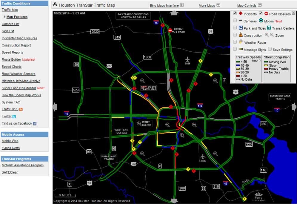
(Source: Texas Department of Transportation (TxDOT)—Houston TranStar®. Last accessed October 28, 2014.)

2.1.1.4 Intelligent Transportation Systems Roadway Detectors

Intelligent Transportation Systems (ITS) roadway detectors are another method of speed data collection. These detector technologies represent traditional monitoring equipment used by public agencies to monitor traffic conditions. Typical ITS detector types include:

• Inductive loops.
• Magnetometer.
• Piezoelectric or bending plates (weigh-in-motion).
• Radar.

These technologies all can provide speed, classification and speed data. Piezoelectric or bending plates also can provide weight information. Speeds can be grouped by classification with these detectors (i.e., speeds for a few length-based truck classes are available). Unlike the methods for speed data collection mentioned up to now, ITS roadway detectors may allow for the measurement of speed information by lane.

A key distinction with these technologies is that speeds are obtained “at a point” rather than direct measurement of travel time along the roadway link of interest as obtained with Bluetooth or toll-tag readers. To obtain travel time from these speeds, the analyst must convert these speeds to a travel time along the link of interest. One typical way to do this is to assume the point speed is representative across the entire link and to divide the link length by the (point) link speed to obtain a travel time along the link of interest.

More details about ITS detector technologies can be found in FHWA’s Traffic Detector Handbook. (Traffic Detector Handbook: Third Edition—Volume I. Federal Highway Administration, Publication No. FHWA-HRT-06-108, October 2006. Traffic Detector Handbook: Third Edition—Volume II. Federal Highway Administration, Publication No. FHWA-HRT-06-139, October 2006.) Another good source for those new to the technologies is the “Equipment” section of the Traffic Monitoring in Federal Lands on-line training. (Traffic Monitoring in Federal Lands. Coordinated Technology Implementation Program (CTIP), Federal Highway Administration Federal Lands Highway Office. 2013.)

2.1.1.5 Electronic License Plate Readers (ELPR)

License plate reader systems are another method for obtaining travel-time information between two points in the roadway network. In this method, license plates are read at one location upstream and then at another location downstream. A time stamp is obtained at both the upstream and downstream location and the difference in these times for matched license plates provide an estimate of the travel time through the link of interest. Character recognition software provides for more automated ELPR. ELPR can be performed manually using tape recorders, portable computers, or video with manual transcription. Data collection and reduction times are more significant with the manual methods.

2.1.1.6 Test-Vehicle Travel Time

In its most manual form, the test-vehicle method of obtaining travel times includes having a driver traverse a corridor while a recorder/observer operates a stopwatch to identify time stamps along particular links of interest along the roadway. Automatic data collection equipment such as a distance measuring instrument (DMI) or GPS facilitate data collection and software can facilitate data reduction and analysis from these automated collection methods.

The “floating car” test-vehicle method employs a driver that “floats” with the traffic stream and attempts to pass as many vehicles as pass the driver. Other test-vehicle methods are available depending upon the application. More information on test-vehicle travel-time data collection is available in Institute of Transportation Engineers (ITE)’s Manual of Transportation Engineering Studies. (Manual of Transportation Engineering Studies, Second Edition. Institute of Transportation Engineers, Washington, D.C., 2010.)

2.1.1.7 Road Tubes

The placement of temporary road tubes with road counters can provide traffic speeds by vehicle classification. Road tubes provide a way to obtain speed (and volume) information for a short-time period (e.g., 48 hours). Speed is obtained by lane through the use of two tubes in the travel direction. Assuming equipment availability, road tubes provide a low-cost way to obtain data. The limitation is that these data are just a sample of traffic speeds and volumes and are not representative of annual conditions. The speeds are just a snapshot, and the volumes require adjustments to estimate annual volume parameters (see section 2.4.3).

2.1.2 Truck Volume Data

Truck volume data can be obtained from a number of sources, some that were described above for travel-time data collection (e.g., ITS detectors). The section below provides more detail on truck volume data sources. Many of the detector technologies for speed (travel time) data only sample vehicles in the traffic stream (e.g., vehicle probes, toll-tag readers, Bluetooth, test vehicles, license-plate readers) so they do not provide traffic volume (or volume by vehicle classification) for the entire traffic stream.

There are generally five possible sources of time-of-day volume data (by vehicle classification) to match to the travel-time data:

1. Classification data for a specific location from a detector (e.g., State department of transportation [DOT] automatic traffic recorders or weigh-in-motion stations).
2. Classification data from a short-term count at a similar and/or adjacent site.
3. Daily volumes (classification) from a roadway inventory database.
4. Classification data from national-level sources from FHWA.
5. Time-of-day volume curves created by vehicle classification.

The following sections describe each of these possible volume data sources in more detail.

2.1.2.1 Roadway Detectors Used for Traffic Monitoring

As described previously, roadway detectors can provide classification data by time-of-day, day-of-week, and/or month-of-year. State DOTs deploy these detectors as part of their routine traffic monitoring activities and include automatic vehicle classification (AVC) and weigh-in-motion (WIM) stations. Most stations are deployed at permanent locations but portable equipment also is used. The main limitation is the number of locations which number in the dozens for small States and the hundreds for large States. Essentially, these are sampling stations that used to develop factors for statewide planning and pavement design.

2.1.2.2 Short-Term Counts

In some cases, the available roadway detectors (AVC, WIM, or others) are not located near the site of the truck bottleneck. In these cases, the analyst may need to collect a short-term count using road tubes or another portable roadway detector technology. These short-term counts are then seasonally adjusted to obtain representative truck counts for the location of interest. More information on seasonal adjustments is described in section 2.4.3. Most States and many local agencies maintain a very large short-term count program but nearly all of the counts are for all vehicles combined, so vehicle classification is not possible.

2.1.2.3 Roadway Inventory Characteristics

State DOTs typically have roadway inventory databases that include geometric and operational aspects of roadways on their maintained system. Analysts can obtain annual average daily traffic (AADT) and truck percentages from these databases to estimate truck volumes for the site of interest. The AADT from these datasets can be adjusted (if necessary) to an hourly value to match the speed (travel time) dataset. The source of the traffic data in these datasets is the roadway detector network discussed immediately above. More information is in sections 2.1.2.5 and 2.4.4.

2.1.2.4 National Sources of Classification Data

National classification datasets are available from FHWA. The source of these data are the State DOT and in some cases local agency traffic monitoring activities; data resubmitted periodically to FHWA. These datasets can provide a consistent source for conducting truck bottleneck studies across States or regions and/or at an area-wide level. The possible FHWA datasets with truck classification data include:

• Highway Performance Monitoring System (HPMS), FHWA Office of Highway Policy Information.
• Vehicle Travel Information System (VTRIS), FHWA Office of Highway Policy Information.
• Travel Monitoring Analysis System (TMAS), FHWA Office of Highway Policy Information.

2.1.2.5 Time-of-Day Truck Volume Curves

Time-of-day truck volume curves can be developed from continuous data sources (e.g., ITS roadway detectors) for planning applications. If built from roadway segments that are similar in geometric and operating characteristics to where they are ultimately applied, they can provide a useful tool. TTI’s Urban Mobility Report uses such profiles created by functional classification, weekend/weekday, and congestion levels (using the speed data) for area-wide congestion statistics and analysis. More information about time-of-day profiles is provided in section 2.4.4.

2.2 Segmentation of Roadway into Reporting Segments

A key element to successful truck bottleneck analysis is the determination of the appropriate segmentation of the roadway network for the desired analyses. To assess the regional nature of truck bottlenecks in an urban area, it is desirable to combine short adjacent links of the roadway network that have similar congestion patterns. By combining short but similar roadway links, one can more easily identify “big picture” urban congestion patterns and the most congested locations in the region. When looking at very detailed congestion data on short links, one can sometimes “miss the forest because of all the trees.” A more focused, follow-up analysis of the most congested locations will likely analyze these shorter links to better understand the specific causes of congestion and possible mitigation strategies.

Therefore, longer segments (composed of short, adjacent links) are recommended for the purposes of regional congestion reporting and identifying potential truck bottleneck locations. Note that this is different from using a long segment that is comprised of a single “data reporting” link; congestion patterns such long segments, common in rural areas, will be diluted by the length making it difficult to identify bottlenecks that may exist on the segment. At least in the former case, the more detailed exists for additional analysis. Traffic levels, congestion patterns, and traffic operation are relatively consistent along these congestion reporting segments (e.g., a defined segment should not include a mix of free-flowing traffic and congested traffic). Ultimately, the use and context of the congestion measures is the key determining factor in the definition of reporting segments. For example, a statewide congestion analysis geared to identifying most congested roadways and truck bottlenecks will likely have longer reporting segments than an arterial street facility-based analysis that is geared toward identifying most congested intersections. The following provides tips for roadway segmentation appropriate for truck bottleneck analyses in urban areas. (Hudson, J. G., N. Wood, B. Dai, and S. M. Turner, 2012 Roadway Congestion Analysis: Performance Report and Information System. Produced by the Texas A&M Transportation Institute for the Capital Area Metropolitan Planning Organization (CAMPO), Austin, Texas, September 2014.)

The segmentation discussion that follows is especially germane for performance reporting, where it is most useful to report performance for roadway facilities. The bottleneck methodology presented in chapter 4 creates segmentation and performance measures based on observed queue lengths for those segments.

2.2.1 For All Roadways

• Short links should be coned into a reporting segment where traffic levels and resulting congestion patterns are relatively consistent.
• Reporting segments are almost always defined uniquely for each direction of travel. The possible exceptions are where: 1) both travel directions have similar congestion patterns; or 2) the scale (e.g., statewide or multi-region) of the analysis is conducive to more aggregate reporting.

2.2.2 Freeways and Access Controlled Highways

• In most cases, a freeway segment will include multiple entrance and exit ramps.
• Freeway segment endpoints are typically entrance or exit ramps from/to another freeway or major cross street, as this is where roadway characteristics, traffic levels, and congestion patterns are most likely to change.
• Freeway segments in dense, built-up areas typically range from 3 to 5 miles in length. These segments also are likely to have more frequent ramp access points.
• Freeway segments in less dense, suburban or exurban areas typically range from 5 to 10 miles in length. These segments are likely to have less frequent ramp access.

2.2.3 Arterial Streets

• In most cases, an arterial street segment will include multiple signalized intersections.
• Arterial street segment endpoints are typically major cross streets, as this is where roadway characteristics, traffic levels, and congestion patterns are most likely to change.
• Arterial street segments in dense, built-up areas typically range from one to three miles in length. These segments also are likely to have higher levels of intersection density.
• Arterial street segments in less dense, suburban or exurban areas typically range from three to five miles in length. These segments are likely to have lower levels of intersection density.

For identifying truck bottlenecks in rural areas, longer reporting segmentation is appropriate (e.g., intercity).

2.3 Quality Control

Prior to data analysis, it is important that the analyst perform quality control of the datasets to ensure certain specifications are met. The quality control process typically includes one or more of the following actions: AASHTO Guidelines for Traffic Data Programs, American Association of State Highway and Transportation Officials, Washington, D.C., 2009.)

1. Reviewing the traffic data format and basic internal consistency.
2. Comparing traffic data values to specified validation criteria.
3. Marking or flagging traffic data values that do not meet the validation criteria.
4. Reviewing marked or flagged traffic data values for final resolution.
5. Imputed marked, flagged, or missing traffic data values with “best estimates” (while still retaining original data values and labeling imputed values as estimates).

The American Association of State Highway and Transportation Officials (AASHTO) Guidelines for Traffic Data Programs (AASHTO Guidelines for Traffic Data Programs, American Association of State Highway and Transportation Officials, Washington, D.C., 2009) describes these quality control processes in more detail. Of particular interest are the definitions for traffic data quality measures, including accuracy, completeness (also referred to as availability), validity, timeliness, coverage, and accessibility (also referred to as usability). More specifically, AASHTO spells out validation criteria for vehicle count, classification, and weight data from ITS detector sources. Additional examples of quality control checks (“business rules”) for ITS detector sources are described elsewhere. (Margiotta, R., T. Lomax, M. Hallenbeck, S. Turner, A. Skabardonis, C. Ferrell, and W. Eisele. Guide to Effective Freeway Performance Measurement: Final Report and Guidebook, National Cooperative Highway Research Program, Washington, D.C., 2006.) Note that some of the prior sections in this section addressed aspects of quality control when the data types were introduced (e.g., Bluetooth).

In some cases, quality control by visual inspection is valuable. Visual inspection is helpful when it is not easy to automate the quality control with business rules. Sometimes the human eye is more adept at identifying reasonableness in data-time series. For example, graphing speed or volume plots by time for a variety of days in the month on the same graphic or looking at lane-by-lane speed and volume relationships on the same graph. Visual inspection of graphics like this allow the analyst to identify places where more “drill down” analyses may be warranted if something suspicious is found. More examples are documented elsewhere. (Margiotta, R., T. Lomax, M. Hallenbeck, S. Turner, A. Skabardonis, C. Ferrell, and W. Eisele. Guide to Effective Freeway Performance Measurement: Final Report and Guidebook, National Cooperative Highway Research Program, Washington, D.C., 2006.)

2.3.1 Probe Speed Data Quality Control

Probe speed data are a very cost-effective source for system-wide data collection. With the increased and widespread use of probe speed data for bottleneck analysis (including truck bottleneck analyses), quality control of these data sources is of particular interest and is the focus of this section. The National Performance Management Research Data Set (NPMRDS) is used as an example in this section to illustrate quality control considerations for a probe speed dataset.

NPMRDS provides travel-time data in five-minute time aggregations. Due to the recent release of NPMRDS, there has been limited investigation of the data source and State DOT and metropolitan planning organization (MPO) practitioners are asking how the dataset can be used for performance measurement and truck analysis on freeways and arterials, and about the general quality of the data for these uses.

As part of an ongoing FHWA Pooled Fund Project (TPF-5[198], Mobility Measurement in Urban Transportation [MMUT]), TTI investigated several States’ worth of the NPMRDS to characterize the roadway coverage, completeness (temporal and spatial), and validity of the five-minute travel-time data. Data for the 14 States in the FHWA pooled fund project at the time of the analysis were included (California, Colorado, Florida, Kentucky, Maryland, Minnesota, New York, North Carolina, Ohio, Oregon, South Carolina, Texas, Virginia, and Washington). Findings are provided here as well as additional analyses related to the truck speed data completeness and validity performed as part of this project. Completeness of the dataset included identification of missing records by traffic message channel (TMC) (the industry standard mapping geography), and by functional classification. For the validity checks, the travel-time data were first converted to speeds, because they can be more intuitively understood and investigated in terms of speed.

Practitioners using large datasets such as NPMRDS for any analyses (such as truck bottlenecks) should understand the data set prior to performing analyses for their specific application. For planning applications, annual averages of five-minute travel-time data may be acceptable rather than day-to-day information that might be more appropriate for operational analyses. Depending upon the application, small nuances in the speeds may not matter, but systematic nuances could cause unacceptable errors.

2.3.1.1 NPMRDS Coverage

The FHWA pooled fund project analysis investigated the coverage of the NPMRDS. Aggregate findings for the United States are summarized in table 1. Analysts investigated the 2011 and 2012 Highway Performance Monitoring System (HPMS) data, and the total directional miles in 2012 on the National Highway System (NHS) increased by 42 percent over 2011 (reflecting the “enhanced NHS” in 2012). Analysts investigated the data from all 13 States in the FHWA pooled fund project, and the entire United States network. Table 1 shows that the U.S. directional-miles of coverage in the 2012 HPMS (NHS) (479,178 directional miles) compares favorably to the NPMRDS network coverage in directional miles (486,953 directional miles).

Analysts took the analysis a step further and put the NPMRDS network on a Geographic Information Systems (GIS) map because that is what is required to perform conflation of speeds and volumes and, again, the results are favorable (475,407 directional miles mapped). The full TMC-encoded network used by industry has approximately 80 percent more coverage (877,882 directional miles—including more arterial/collector coverage) than the NPMRDS network across the United States.

The coverage results of the individual States were generally the same as those documented in table 1 for the United States.

Table 1. United States traffic message channel—Roadway coverage in National Highway System and National Performance Management Research Data Set.

2012 HPMS NHS (Directional Miles)	NPMRDS Network (Directional Miles)	NPMRDS GIS/Map Network (Directional Miles)	Full TMC Network (Directional Miles)
479,178	486,953	475,407	877,882

(Source: Adapted from Information Sharing on FHWA’s NPMRDS, Webinar. Texas A&M Transportation Institute, FHWA Pooled Fund Project: Mobility Measurement in Urban Transportation, April 2014.)

2.3.1.2 NPMRDS Completeness

The NPMRDS is five-minute travel-time data for each day and data are present only when probe vehicles are present (i.e., data are not estimated when missing). Therefore, it is important for analysts to understand how incomplete data may affect analyses and measure calculation. The analyst should ask himself or herself what level of completeness is needed for their performance measure application. The analyst may need to impute missing values on specific days of interest. If overall performance for extended periods of time is needed, aggregated statistics to monthly, quarterly, or even annually for day of week may be acceptable.

NPMRDS provides three travel-time values for each five-minute time period and TMC: 1) mixed vehicle; 2) passenger car; and 3) truck. Analysts investigated the completeness of mixed-vehicle and truck travel-time values in the dataset. A three-month dataset from November 2013 to January 2014 was used for the analysis. Daylight hours were used for analysis (6:00 a.m. to 8:00 p.m.) because most analysis are most concerned with daytime traffic conditions, rather than overnight hours. (Nighttime travel is important for trucks, but there is less interference from passenger cars then.) Analysts looked at three aggregation-time periods of results: 1) individual day-to-day; 2) one-month average day-of-week; and 3) three months day-of-week.

Completeness in number 3 (three months day-of-week) was satisfied if any five-minute travel-time value was present for the given TMC for the given five-minute time period over the three-month period. Similarly, the one-month average day-of-week was satisfied if a travel-time value was present for the given TMC over the one-month time period. The individual day-to-day value represents the percentage of time the data were available for the specific five-minute time period of interest.

Analysts also aggregated the 5-minute data to 15-minute time periods, urban versus rural and roadway functional classification. The average completeness values for mixed traffic and trucks are shown as rows in table 2. The results in table 2 are average completeness estimates across the 13 States represented in the FHWA pooled fund project.

The above analysis is only a snapshot for a specific time period. It is important to note that the NPMRDS, as well as other commercial data sources, will continue to evolve over time. The authors expect, but cannot be absolutely certain, that data quality and completeness will improve over time. For example, starting in February 2014, an effort is underway to increase the truck data within the NPMRDS dramatically. However, users should still be cautious in using third-party data, and replicating the above quality and completeness analyses is a sound first step before embarking on analysis.

Table 2. Completeness percentages for the National Performance Management Research Data Set for mixed traffic and trucks.
(Note: All NHS/NPMRDS (Daytime only, 6:00 a.m. to 8:00 p.m.); average completeness values of 14 States represented in the FHWA MMUT Pooled Fund Project; three months of data from November 2013 to January 2014.)

Travel-Time Type	Urban/Rural	Functional Classification	Individual Day-to-Day— 5 minutes	Individual Day-to-Day— 15 minutes	One Month—Average Day-of-Week— 5 minutes	One Month—Average Day-of-Week— 15 minutes	Three Months—Average Day-of-Week— 5 minutes	Three Months—Average Day-of-Week— 15 minutes
Mixed-Vehicle	Urban and Rural	All NHS	28% (About 28 percent is based on 583,070,592 observations out of a total of 2,053,298,688.)	48%	58%	76%	78%	90%
Mixed-Vehicle	Urban	Class 1—Interstate	54%	76%	82%	93%	95%	98%
Mixed-Vehicle	Urban	Class 2—Other Freeway/Expressway	36%	61%	71%	88%	91%	97%
Mixed-Vehicle	Urban	Class 3 and 4—Principal/Minor Arterial	23%	44%	55%	77%	81%	93%
Truck	Urban and Rural	All NHS	6% (About 6 percent is based on 128,723,738 observations out of a total of 2,053,298,688.)	15%	30%	33%	48%	67%
Truck	Urban	Class 1—Interstate	19%	33%	58%	67%	81%	91%
Truck	Urban	Class 2—Other Freeway/Expressway	6%	13%	3%	39%	60%	79%
Truck	Urban	Class 3 and 4—Principal/Minor Arterial	3%	5%	16%	21%	37%	60%

(Source: Adapted from Information Sharing on FHWA’s NPMRDS, Webinar. Texas A&M Transportation Institute, FHWA Pooled Fund Project: Mobility Measurement in Urban Transportation, April 2014 and original analysis for this report.)

The completeness results in table 2 lead to the following observations:

• Aggregation from individual day to monthly or quarterly increases completeness.
• Aggregation from 5-minute data to 15-minute data increases completeness.
• Truck data completeness percent is substantially less than mixed vehicle.
• Completeness decreases with decreasing functional classification.
• Completeness in urban areas is generally slightly higher than in rural areas (documented elsewhere). (Information Sharing on FHWA’s NPMRDS, Webinar. Texas A&M Transportation Institute, FHWA Pooled Fund Project: Mobility Measurement in Urban Transportation, April 2014.)

These NPMRDS completeness results suggest the analyst should recognize that the five-minute travel-time data are thin in some cases, particularly for the truck data and particularly on principal and minor arterials. Analysts should use caution and be careful not to “slice the data too thinly” for certain performance activities such as planning-level analysis, including many truck bottleneck studies. While analyses were conducted using the NPMRDS for this study, it is highly likely that other third-party travel-time data show similar tendencies, highlighting the need for users to scrutinize the data before conducting analyses. It should be noted that aggregation is one method for practitioners to handle missing data, and imputation is another. These observations also pertain to historical data; future data will likely show higher completeness rates. Imputation methods could look at time slices before/after the missing data and/or look at adjacent days. Imputation has been accomplished through a variety of methods, but they are all imperfect (See, for example, the SHRP Project L02 Report and Guidebook). If imputation is done, analysts must clearly document: 1) the amount of data that has been imputed by time period; and 2) details of the imputation methodology.

2.3.1.3 National Performance Management Research Data Set Validity

Analysts performed a validity test of NPMRDS meant to verify how often speeds were in a specific range or how often there were notable differences between the car and truck travel-time data. As mentioned previously, the five-minute travel-time data from NPMRDS were converted to speeds and the following validity tests were investigated by functional classification:

• Percent of mixed-vehicle speeds and truck speeds less than 5 miles per hour by functional classification (table 3).
• Percent of mixed-vehicle speeds and truck speeds greater than 75 miles per hour by functional classification (table 3).
• “Car minus truck speed” difference cumulative percentage distribution by functional classification (figures 2 through 4).

Table 3. Mixed speed and truck speed percentage validation results by functional classification.
(Note: All NHS/NPMRDS (Daytime only, 6:00 a.m. to 8:00 p.m.); average validity values of 14 States represented in the FHWA Pooled Fund Project; one month of data used in the analysis (January 2014).)

Validity Check	Speed Data Type	Functional Classification	Percentage
Speed <5 miles per hour	Mixed-vehicle	Interstate	0%
Speed <5 miles per hour	Mixed-vehicle	Other Freeway and Expressway	0%
Speed <5 miles per hour	Mixed-vehicle	Principal and Minor Arterials	3%
Speed <5 miles per hour	Truck	Interstate	0%
Speed <5 miles per hour	Truck	Other Freeway and Expressway	1%
Speed <5 miles per hour	Truck	Principal and Minor Arterials	2%
Speed >75 miles per hour	Mixed-vehicle	Interstate	1%
Speed >75 miles per hour	Mixed-vehicle	Other Freeway and Expressway	1%
Speed >75 miles per hour	Mixed-vehicle	Principal and Minor Arterials	0%
Speed >75 miles per hour	Truck	Interstate	0.08% (0.08% is based on 18,510 observations out of a total of 23,474,056 observations.)
Speed >75 miles per hour	Truck	Other Freeway and Expressway	0.03% (0.03% is based on 1,153 observations out of a total of 4,568,560 observations.
Speed >75 miles per hour	Truck	Principal and Minor Arterials	0.05% (0.05% is based on 5,526 observations out of a total of 10,542,144 observations.)

(Source: Adapted from Information Sharing on FHWA’s NPMRDS, Webinar. Texas A&M Transportation Institute, FHWA Pooled Fund Project: Mobility Measurement in Urban Transportation, April 2014 and original analysis for this report.)

Figure 2. Graph. “Car speed minus truck speed” difference cumulative percentage distribution, Interstates.
(Note: All NHS/NPMRDS (Daytime only, 6:00 a.m. to 8:00 p.m.); average validity values of 14 States represented in the FHWA Pooled Fund Project; one month of data used in the analysis (January 2014).)

(Source: Original analysis of FHWA Pooled Fund Project: Mobility Measurement in Urban Transportation data for this report.)

Figure 3. Graph. “Car speed minus truck speed” difference cumulative percentage distribution, other freeway and expressway.
(Note: All NHS/NPMRDS (Daytime only, 6:00 a.m. to 8:00 p.m.); average validity values of 14 States represented in the FHWA Pooled Fund Project; one month of data used in the analysis (January 2014).)

(Source: Original analysis of FHWA Pooled Fund Project: Mobility Measurement in Urban Transportation data for this report.)

Figure 4. Graph. “Car speed minus truck speed” difference cumulative percentage distribution, principal and minor arterials.
(Note: All NHS/NPMRDS (Daytime only, 6:00 a.m. to 8:00 p.m.); average validity values of 14 States represented in the FHWA Pooled Fund Project; one month of data used in the analysis (January 2014).)

(Source: Original analysis of FHWA Pooled Fund Project: Mobility Measurement in Urban Transportation data for this report.)

The validity results in table 3 generally indicate low occurrences of the validity checks being satisfied. Other results appear less intuitive (i.e., differences between car speeds and truck speeds, particularly when trucks are faster). For example, on Interstates and other freeways and expressways (figures 2 and 3), approximately 5 percent of data have truck speeds 10 miles per hour faster or more than cars. For principal and minor arterials (figure 4), approximately 10 percent of the data have truck speeds 10 miles per hour faster or more than cars. Depending upon functional classification, between 25 percent and 35 percent of the data indicate truck speeds faster than car speeds.

The relatively low occurrences documented in table 3 and figures 2 through 4 may not impact overall results, but analysts should run such validity tests to verify if/when they do occur and whether they occur during a time period that could impact the results for their specific application (e.g., truck bottleneck analysis).

Because NPMRDS travel-time data exist at the five-minute level, the analyst should verify that adequate travel-time data sample is available for the analyses desired. As described in the prior section, in some cases the travel-time samples at five minutes are limited (particularly the truck-only travel-time data). To obtain adequate NPMRDS travel-time data sample for a particular analysis, the analyst may need to do the following (for TMCs of interest):

• Aggregate the 5-minute travel-time data to a 15-minute or hourly travel-time estimate.
• Aggregate the daily travel-time data to a monthly, seasonal, or yearly travel-time estimate.
• Impute data from adjacent-time periods and/or adjacent days.

2.3.1.4 Concluding Thoughts for Practitioners

The following are two important questions the analyst should ask himself or herself to determine the most appropriate aggregation level of the NPMRDS travel-time data:

• What temporal aggregation is necessary for decision-makers using the results of this analysis? For example, for a planning study, it is possible that seasonal or annual statistics summarized from 15-minute or hourly data will be adequate.
• What spatial aggregation is necessary for decision-makers using the results of this analysis? The travel-time data from NPMRDS begin at the TMC level. In rural areas, TMCs are typically very long while in urban areas they can be shorter (e.g., ramp-to-ramp on an Interstate). It is likely that the analyst will want to perform segmentation of their roadway network for analysis differently than the TMC level. Segmentation is described in more detail in section 2.2.

After determining the appropriate temporal and spatial aggregation of the NPMRDS travel-time data (or by imputation), it is recommended that the analyst convert the travel-time information to speeds for quality control prior to aggregation. Within the NPMRDS, there is an inventory file with TMC segment information, including length (miles), a road label (description) and GPS x-y coordinates for the start and endpoints of the TMC. The TMC length (miles) divided by the travel time (in seconds) multiplied by 3,600 (seconds in an hour) gives the speed (miles per hour) for the TMC of interest.

Reviewing speeds is more intuitive for recognizing suspicious speed data and performing quality control. The analyst may want to remove (or cap) speeds that are unreasonably high. An appropriate speed cap, if desired, should consider the functional classification of the roadway (freeway or arterial) and the speed data being investigated (“truck” or “passenger car” or “all vehicles”). After quality control of the data, average speeds are computed for the temporal and spatial aggregation levels desired.

2.4 Data Processing Procedures to Match Travel-Time (Speed) and Volume Data Sources

2.4.1 Implications of Application

The ultimate use/application of the output from an analysis drives the data processing procedures, as well as data collection and data reduction decisions. The primary application for this methodology is the determination of truck bottlenecks for prioritizing investment decisions. While that sounds straightforward, there are still important considerations for the data analyst that will impact data collection, data reduction, and data processing steps.

Ultimately, public-sector transportation professionals are trying to make the best decisions in the most cost-effective manner possible, given the available data. It is not always possible to obtain data at the spatial and temporal granularity for the specific location(s) of interest. Table 4 illustrates the spatial and temporal data availability tradeoffs that are rather commonplace in performing truck bottleneck studies when complete data are not available.

Table 4. Speed and volume spatial and temporal data availability considerations.

	Data Availability—Spatially	Data Availability—Temporally
Most desirable are…	…actual data for the specific site(s) of interest…	…and/or data at desired time granularity to satisfy the application (e.g., annual, hourly, 15-minute, 1-minute).
Less desirable are…	…estimated data from similar site(s)…	…and/or data aggregated over time because desired granularity not available.

(Source: Cambridge Systematics, Inc.)

2.4.2 Use of Paired Speed-Volume Observations from Intelligent Transportation Systems Detectors

Many public transportation agencies have roadway ITS detectors to monitor traffic conditions and operate the transportation system. The benefit of these detectors is that they typically can provide very disaggregate data (lane-by-lane, minute-by-minute) for a specific location. These data are the “most desirable” as shown in table 4. If that location is the specific location for which a truck bottleneck is of interest, the analyst benefits from having very good speed and volume information for analysis and decision-making. These data are sometimes called “paired speed-volume observations” because the speed and volume data are collected and available over the same time period. The analyst can then begin to develop the bottleneck performance measures as described in more detail in section 4.4.

For truck bottleneck analysis (and prioritization), it is important to ensure that the “paired speed-volume observations” occur over a “representative” time period for the locations of interest. This ensures that they will not rank artificially higher (if measured during a highly congested month/season) or artificially lower (if measured during a relatively low-congestion month/season). Adjustment factors for factor groups and/or representative sites to the data collection site can aid in selection of the “representative” time period to target for analysis. More information on adjustment factors are described in the next section.

2.4.3 Assigning Short-Term Volume Count to Continuous Travel-Time Data

Another common data scenario is when traffic volumes are available from a short-term volume count (e.g., 48 hours) and continuous travel-time data are available from a commercial source. Continuous means that the travel-time data are available throughout the year (e.g., for each five-minute period such as NPMRDS). A short-term volume count typically implies data are obtained by road tubes or some other means.

As discussed, the application here is summarizing annual bottleneck statistics to prioritize truck bottleneck areas. In this case, there is a need to “adjust” the short-term truck volume count to the same granularity of the travel-time data, which are available throughout the year in this example. The short-term volume count must be adjusted seasonally (hour-of-day, day-of-week, and month-of-year).

The following procedure from the AASHTO Guidelines for Traffic Data Programs can be used to convert a short-term volume count (with at least 24 hours of data) into an estimate of AADT: (AASHTO Guidelines for Traffic Data Programs, American Association of State Highway and Transportation Officials, Washington, D.C., 2009.)

1. Summarize the count as a set of hourly counts.
2. Divide each hourly count by the appropriate seasonal traffic ratio (or multiply by the appropriate seasonal traffic factors).
3. For each hour of the day, average the results of step 2, producing 24 hourly averages; and sum the 24 hourly averages to produce estimate AADT.

This procedure assumes traffic factors are available from continuous monitoring sites that are the reference site for the segment of interest. Traffic volume by vehicle class (e.g., single-unit and combination trucks) is estimated using a similar procedure where the factors used in step 2 are those developed by vehicle classes of interest. More details about this procedure are available elsewhere. (AASHTO Guidelines for Traffic Data Programs, American Association of State Highway and Transportation Officials, Washington, D.C., 2009. Traffic Monitoring Guide, Federal Highway Administration, September 2013.)

2.4.4 Deriving Detailed Volume and Vehicle Class Estimates to Match the Level of Detail in the Travel-Time Dataset

In some situations, travel-time data are available for 15-minute or hourly time periods aggregated for an entire year (e.g., average speed or travel time for a roadway segment for the 52 Mondays of the year between 7:00 and 7:15 a.m.), while only an AADT and associated truck percentage are available for volumes. In these cases, there is the need to derive detailed volume and vehicle class estimates to match the level of detail in the travel-time dataset.

One approach for dividing the daily traffic count into the same-time interval as the speed dataset (5-minute, 15-minute, or hourly) has been created by the Texas A&M Transportation Institute (TTI) for the list of 100 Most Congested Roadways produced for the Texas Department of Transportation (TxDOT). (100 Most Congested Roadways, Texas Department of Transportation, August 31, 2014. Most Congested Roadways in Texas, Texas A&M Transportation Institute, August 31, 2014.) A similar method is used in TTI’s Urban Mobility Report. (Schrank, D. L., T. J. Lomax, and B. Eisele, 2012 Urban Mobility Report. December 2012.)

The following sections describe the procedural steps used to divide the daily traffic counts into the same temporal scales as the travel-time data for the 100 Most Congested Roadways list.

2.4.4.1 Step 1—Identify Traffic Volume Data

The Roadway-Highway Inventory Network (RHiNo) dataset from TxDOT provides the source for traffic volume data, although the geographic designations in the RHiNo dataset are not identical to those used for the private-company speed data. While there are some detailed traffic counts on major roads, the most widespread and consistent traffic counts available are AADT counts. The 15-minute traffic volumes for each section, therefore, were estimated from these AADT counts using typical time-of-day traffic volume profiles developed from local continuous count locations (e.g., ITS detectors).

Truck volumes are calculated in the same way by applying the truck-only 15-minute volume profiles to the truck AADTs reported in RHiNo. These 15-minute truck volumes were split into values for combination trucks and single-unit trucks using the percentages for each from RHiNo. These truck-only profiles account for the fact that trucks volumes tend to peak at very different rates and times than do the mixed-vehicle traffic.

Volume estimates for each day of the week (to match the speed database) were created from the annual average volume data using the factors in table 5. Automated traffic recorders from the Texas metropolitan areas were reviewed and the factors in table 5 are a “best-fit” average for both freeways and major streets. Creating a 15-minute volume to be used with the traffic speed values, then, is a process of multiplying the annual average by the daily factor (table 5) and by the 15-minute factor (figures 5 and 6 described in section 2.4.4.3).

Table 5. Day-of-week volume conversion factors.

Day of Week	Adjustment Factor (to Convert Average Annual Volume into Day-of-Week Volume)
Monday to Thursday	+5%
Friday	+10%
Saturday	-10%
Sunday	-20%

(Source: Adapted from: 100 Most Congested Roadways, Texas Department of Transportation, August 31, 2014; and Schrank, D. L., T. J. Lomax, and B. Eisele, 2012 Urban Mobility Report. December 2012.)

2.4.4.2 Step 2—Combine the Road Networks for Traffic Volume and Speed Data

The second step was to combine the road networks for the traffic volume and speed data sources, such that an estimate of traffic speed and traffic volume were available for each desired roadway segment. The combination (also known as conflation) of the traffic volume and traffic speed networks was accomplished using GIS tools. See section 2.4.5 for additional information about conflation. The TxDOT traffic volume network (RHiNo) was chosen as the base network; a set of speeds from the speed network was applied to each segment of the traffic volume network. Multiple RHiNo segments make up a section in the 100 Most Congested Roadways list.

2.4.4.3 Step 3—Estimate Traffic Volumes for Shorter-Time Intervals

The third step was to estimate passenger car and truck traffic volumes for the 15-minute time intervals. The process includes the following:

• A simple average of the 15-minute traffic speeds for the morning and evening peak periods was used to identify which of the time-of-day volume pattern curves to apply. The morning and evening congestion levels were an initial sorting factor (determined by the percentage difference between the average peak-period speed and the free-flow speed).
• The most congested period was then determined by the time period with the lower speeds (morning or evening); or if both peaks have approximately the same speed, another curve was used. Sample traffic volume profiles are shown in figure 5.
• Low, medium, or high congestion levels—The general level of congestion is determined by the amount of speed decline from the off-peak speeds. Lower congestion levels typically have higher percentages of daily traffic volume occurring in the peak, while higher congestion levels are usually associated with more volume in hours outside of the peak hours.
• Morning or evening peak; or approximately even peak speeds—The speed database has values for each direction of traffic and most roadways have one peak direction. This identifies the time periods when the lowest speed occurs and selects the appropriate volume distribution curve (the higher volume was assigned to the peak period with the lower speed). Roadways with approximately the same congested speed in the morning and evening periods have a separate volume pattern; this pattern also has relatively high volumes in the mid-day hours.
• Separate 15-minute traffic volumes for trucks and non-trucks were created from the 15-minute traffic volume percentages generated from profiles such as figure 5 (mixed traffic) and figure 6 (truck).

Figure 5. Graph. Weekday mixed-traffic distribution profile for no to low congestion.

(Source: Adapted from 100 Most Congested Roadways, Texas Department of Transportation, August 31, 2014; and Schrank, D. L., T. J. Lomax, B. Eisele, 2012 Urban Mobility Report, December 2012.)

Figure 6. Graph. Weekday freeway truck-traffic distribution profiles.

(Source: Adapted from 100 Most Congested Roadways, Texas Department of Transportation, August 31, 2014.)

2.4.5 Conflation Procedures

“Conflation” is the process of matching probe speed data to roadway volume data. It is necessary for computing performance measures for truck bottleneck analysis when the speed and roadway volume data are provided on different networks.

The first step in the conflation process is determining which roadway network will serve as the base network for conflation. The base network is the roadway network, which gets the attributes from the other network loaded on it. Generally, the base network should be the network that more closely aligns with the purpose for the analysis. Because datasets are large and processing time can be lengthy, it is important to consider if any records can be eliminated (i.e., by excluding some functional classes to speed processing time).

The process of conflation is facilitated by using GIS to import and compare the end points of the speed data roadway network with the traffic volume inventory. Quality control is a necessary step to ensure that the data from the speed network aligns with the volume network. More information on conflation can be found elsewhere. (Schrank, D. L., “Conflation Procedure to Combine Speed and Volume Datasets for MAP-21 Performance Measurement.” Presentation at the North American Travel Monitoring Exposition and Conference (NATMEC) 2014, Chicago, Illinois.) The basic principles of conflating vehicle probe data to agency data bases are as follows.

2.4.5.1 Step 1—Build a Route System

At the center of the methodology is the need to reference both datasets segments against a common road network. As such, a base road network to which the data will be conflated and an associated route system is required. The base road network must be topologically connected (i.e., does not contain gaps at intersections) and should not contain overlaps to allow for network tracing.

2.4.5.2 Step 2—Conflate Data

The data is conflated to the base road network by snapping the end points of the polyline to the network, and then determining the logical road network link(s) that form the path between the two points. This path is output as one or more linear events giving the Route ID and the route measures at the ends of the event.

In this process, it is assumed that the polylines are digitized in the direction of travel, and the ends of the polylines must be spatially accurate enough to allow them to be snapped to the routes using a reasonable snapping tolerance.

In the snapping process:

1. If both end points snap to the same route, it is assumed this is the best path and a single linear event is generated.
2. If the end points snap to the adjacent routes, it is assumed this is the best path and two linear events are generated.
3. If there is no obvious path between the two point, network tracing is used to determine the shortest path between the points taking into account direction of travel on the network. Assuming the length of the calculated path is similar (i.e., within a defined percentage of) the length of the original polyline, it is assumed to be a match and multiple linear events are generated.

The results of this step is a linear event table referenced against the route system developed in step 1 containing (at least) the following fields:

RouteID—Unique route ID

FrMeasure—From measure

ToMeasure—To Measure

{PolylineID}—A unique ID for the polyline

2.4.5.3 Step 3—Event Overlay

To generate the many-to-many relationship table between the two datasets, the two linear event tables generated from the two datasets in step 2 must be overlaid against each other to determine the unique overlaps in the events, and for each of these overlaps the length the overlap.

The results of this event overlay step is a single linear event table containing (at least) the following fields:

RouteID—Unique route ID

FrMeasure—From measure

ToMeasure—To Measure

Length—Length, in map units, of the linear event

{Polyline1ID}—ID of the polyline from dataset 1

POverlap1—Percentage overlap, based on length, between the original polyline from dataset 1 and the linear event

{Polyline2ID}—ID of the polyline from dataset 2

POverlap2—Percentage overlap, based on length, between the original polyline from dataset 2 and the linear event

2.4.5.4 Step 4—Join

To allow data in the two datasets to be compared against each other, the two original datasets must be joined to the linear event table generated in step 3. This will produce a single linear event table containing the attributes of both datasets. Note: If any attributes need to be apportioned (e.g., travel time), this can be accomplished using the “POverlap1” and “POverlap2” event table attributes.

You may need the Adobe® Reader® to view the PDFs on this page.

previous | next