Transportation Systems Management and Operations Benefit-Cost Analysis CompendiumCHAPTER 7. DEMAND MANAGEMENT
Case Study 7.1 – Minnesota I-35W Urban Partnership
Note: Chapters 2, 3, and 4 of this Compendium contain a discussion of the fundamentals of benefit-cost analyses (BCA) and an introduction to BCA modeling tools. These sections also contain additional BCA references. Project Technology or Strategy
This case study and all tables and data are taken directly from Appendix J of Urban Partnership Agreement: Minnesota Evaluation Report, http://www.dot.state.mn.us/rtmc/reports/
hov/20130419MnUPA_Evaluation_Final_Rpt.pdf In 2006, the U.S. Department of Transportation, in partnership with metropolitan areas, initiated a program to explore reducing congestion through the implementation of congestion pricing activities combined with necessary supporting elements. This program was instituted through the Urban Partnership Agreements (UPA) and the Congestion Reduction Demonstrations (CRDs). Minneapolis, Minnesota was selected for a UPA award. The projects under the Minnesota UPA focused on reducing traffic congestion in the I-35W corridor and in downtown Minneapolis. I-35W South is the section south of downtown Minneapolis and I-35W North is the section north of downtown Minneapolis. The Minnesota UPA included 24 projects. A major focus of the Minnesota UPA was on reducing congestion on I-35W South. As a result, the Minnesota UPA Benefit-Cost Analysis (BCA) focused on projects associated with I-35W South. Table 33 describes the projects associated with I-35W South that were included in the BCA and how the portion of the costs included in the BCA were determined.
Source: Federal Highway Administration
Three Minnesota UPA projects were not included in the BCA because they are on I-35W North, outside the main UPA focus corridor of I-35W South. The projects not included in the BCA are the I-35W North and 95th Avenue park-and-ride lot expansion, the new park-and-ride lot at I-35W North and County Road C, and the real-time traffic and transit information signs along I-35W North. Project Goals and ObjectivesThe addition of the MnPASS HOT lanes, the PDSL, the new and expanded park-and-ride lots, the new bus routes, the new auxiliary lanes on I-35W South, and the MARQ2 lanes in downtown Minneapolis provided additional capacity on I-35W South and travel options for users. The new general-purpose freeway lanes in the Crosstown Commons section, which were not part of the UPA, also added capacity and, along with other improvements in this section, eliminated a major bottleneck on the freeway. All of these improvements were expected to result in increased travel speeds, reduced travel times, and increased throughput. DataThe BCA for the Minnesota UPA projects used several data sources:
Minnesota UPA Projects – CostsData on the capital costs, the implementation costs, the operating and maintenance costs, and the replacement and re-investment costs for the projects were obtained from MnDOT and Metro Transit. To convert any future year costs to year 2009 dollars, a real discount rate of 7 percent per year was used (based on guidance from http://www.whitehouse.gov/omb/assets/a94/a094.pdf (page 9) and current FHWA guidance (Federal Register, Vol. 75, No. 104, p. 30476)). A 10-year post-deployment timeframe was used for the BCA since many aspects of the projects were technology- or pricing-related. Both technology and pricing systems have relatively short life spans. Thus, only expenditures prior to December of 2019 incurred as a result of implementing the UPA projects were considered. In addition, only the marginal costs associated with the UPA projects and the reconstruction of the Crosstown Commons section were included in the cost data. The BCA timeframe began with the first expenses incurred and ends in 2019, after 10 years of operations. The Minnesota UPA projects with useful lives longer than 10 years, such as new park-and-ride lots or new HOT lanes, were accounted for by including their salvage value in year 10. The U.S. DOT allocated $133.3 million for the Minnesota UPA projects. The state of Minnesota funded the eWorkPlace telecommuting program. The funding was used to plan, design, and construct the various projects. Operating and maintaining the projects over the BCA timeframe of 10 years will require additional funding. To address costs incurred in years other than 2009, those costs were adjusted to a common year using a discount rate of 7 percent. Therefore, determining the costs of the UPA projects was more difficult than simply assuming that the costs total $133 million. Table 34 describes the costs associated with the Minnesota UPA BCA.
1 There will be a small reinvestment cost ($2,400) for lane guidance equipment in the year 2015. For simplicity this has been added to the operations and maintenance costs.
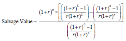
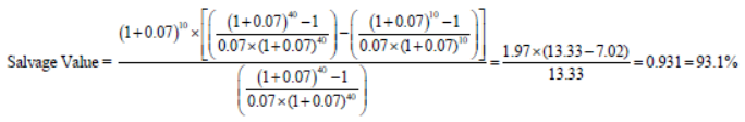
In December 2019 some of the above items will still have value, which is known as salvage value. The salvage value will be subtracted from the total cost above (approximately $395,156,082) to determine the cost over the 10 year BCA timeframe. The electronic components of the DAS for shoulder-running buses, real-time transit and next bus arrival information, transit signal priority along Central Avenue, the telework program, and the real time traffic informational signs were assumed to have negligible salvage value at the end of 10 years. For the physical infrastructure (HOT lane, PDSL, P&R lots, MARQ2, and Transit Advantage Lane) Minnesota's BCA guidance was used (http://www.dot.state.mn.us/planning/program/benefitcost.html) to obtain the salvage value using the following formula: Figure 32. Equation. Salvage Value. Where r = the discount rate (0.07) This same guidance suggests the useful life of surface (pavement) is 25 years, sub-base and base are 40 years, and major structures have longer timeframes. Since many of these items are additional lanes or parking lots, a life span of 40 years was chosen. The salvage value is therefore: Figure 33. Equation. Salvage Value Calculated Using Minnesota Urban Partnership Agreement Data. Salvage Value = 93.1% × ($39,616,038 × $31,707,815 × $33,405,610 × $714,779 + $228,000,000) × 93.1% × $333,444,242 = $310,367,064 The one remaining item is the salvage value of the 27 new buses after 10 years of service. Assuming that the buses have a useful life of 12 years then the salvage value equals: $3,668,514 × 22.8% = $835,075. Therefore, the resulting 10-year costs from the Minnesota UPA projects were $395,156,082 − $310,367,064 − $835,075 = $83,953,942. BenefitsThe benefits of the Minnesota UPA projects are similar to benefits from many transportation infrastructure projects and the calculation methodology will follow standard practice (http://bca.transportationeconomics.org/). This section highlights how the benefits were calculated for the UPA projects. The preferred option to estimate the impacts, and therefore benefits, of the UPA projects was to use the Metropolitan Council's urban planning model. Unfortunately, the output from the model for the year 2010 for I-35W South was considerably different than results recorded in the field based on data from Minnesota's extensive loop detector system. For example, the model output showed considerable congestion during the morning and evening peak period where actual data showed only minor congestion. Travel speeds in the model were between 10 mph to 30 mph slower than actual speeds (depending on direction, segment of I-35W and time of day). Thus, the model could not be expected to accurately capture the change in travel conditions caused by the UPA projects. Additionally, the amount of modifications and calibrations that would have been required to adjust model outputs to real world results would have yielded a model that was so altered that it could no longer be expected to properly estimate the impacts of the UPA projects. Using actual data to estimate the impact of the UPA projects has one main advantage – it is the true data but has several disadvantages. The main disadvantages are (1) the impact of exogenous factors, for example the price of gas impacting travel or the new cross town connector, cannot be properly excluded and (2) actual data is good only for the year it was collected and impacts in future years must be estimated. An assumption was made that the impacts observed in the first year post- deployment will remain constant over the 10-year timeframe. In theory, using year one changes would represent a conservative estimate of benefits since many key benefits of the UPA projects would increase over time given the expected continued increase in regional traffic volumes and health care costs (which will equate to greater benefits associated with emissions reductions). Finally, since the reconstruction of the Crosstown Commons section occurred at the same time as the UPA projects, it was impossible to separate the impacts (benefits) of the UPA projects from the Crosstown Commons section reconstruction. Therefore, the benefits outlined below are likely due to the UPA projects and the Crosstown Commons section reconstruction. As a result, the costs of both the UPA projects and the Crosstown Commons section were included in the BCA. Travel Time SavingsThe amount of time saved by travelers was converted to monetary benefits based on FHWA guidance (Table 4 in https://www.transportation.gov/sites/dot.gov/files/docs/USDOT%20VOT%20Guidance%202014.pdf). The value of time for the year 2009 was $12.50 based on local travel, weighted by the average of both business and other travel. This value was adjusted for future values of time by increasing it by 1.6 percent per year (prior to applying the discount rate) as outlined in the FHWA document https://www.transportation.gov/sites/dot.gov/files/docs/USDOT%20VOT%20Guidance%202014.pdf. Travel time data for travelers on I-35W South was obtained from MnDOT's extensive system of loop detectors and analyzed as part of the traffic data analysis conducted as part of the UPA evaluation. These detectors provided a reliable source of data to determine travel speeds pre- and post-deployment of the UPA projects. The pre- deployment data used in the congestion analysis covered the period from October 2008 to April of 2009 and the post-deployment data covered the period from December 2010 to October 2011. The loop detector data was obtained from the following three sections of I-35W South for the congestion analysis.
Only peak periods travel times were included in the analysis. The UPA projects were expected to have minimal to no impact on travel times in off peak periods as those travel times were already free- flow. The travel time savings are shown in Table 35.
Note: Negative values indicate an increase in travel time after the UPA projects.
Source: Federal Highway Administration The next step in the BCA was to determine the number of vehicles that obtained these travel time savings. Existing (before UPA projects) travelers will receive the travel time savings shown in Table 36. New vehicles (induced demand due to improved traffic flow) would not necessarily gain the entire savings based on their previous travel. To induce these new travelers, this route may save them anywhere from almost no time up to almost the full time savings shown in Table 35. It was generally assumed that a reasonable estimate is that half the time shown in Table 35 was saved by additional vehicles to the roadway. Finally, the total vehicle hours of travel time savings was obtained using the following calculation: Travel Time Saved = (Before Volumes) × (Travel Time Savings) + (Volume Change) × (0.5 x Travel Time Savings) Figure 34. Equation. Total Vehicle Hours of Travel Time Savings. Total time savings for all time periods amounted to 1,255 vehicle- hours in the morning and 2,987 vehicle hours in the afternoon. This figure was multiplied by the number of days per year with congestion (Monday through Friday minus holidays, approximately 254 per year) resulting in 1,077,324 vehicle-hours per year saved on I-35W South. These 1,077,324 vehicle-hours were then split into trucks (heavy vehicles) and automobiles. According to MnDOT, during the peak periods trucks represent 8.1 percent of traffic on I-35W South. Therefore, there were 87,263 truck-hours of delay and 990,061 automobile-hours of delay. The automobile delay was then adjusted to person-hours based on average vehicle occupancy (AVO) on I-35W of 1.1 during the peak periods. This figure was provided by MnDOT. The resulting total savings of 1,089,067 person-hours of delay was for automobiles. These savings were assumed to continue from 2010 to 2019. The saved travel times were then multiplied by the value of time for trucks ($24.70/hour) and automobile travelers ($12.50/hour) (adjusted to 2009 values), resulting in a total benefit of $139,474,650 (in 2009 dollars). The methodology to calculate the value of travel time savings obtained by transit riders was similar to that of automobile travelers. Additionally, the value of their time was identical to what was outlined for automobile travelers. In this case the number of transit riders before and after the UPA projects, along with their travel time savings, was obtained from the transit analysis in Appendix C of the Minnesota UPA Evaluation – Transit Analysis. There was almost no change in the number of riders from 2009 to 2011 on I-35W South. The morning peak period increased from 4,814 riders per day to 4,859 riders per day. The afternoon peak increased from 4,592 riders per day to 4,602 riders per day. For existing (2009) riders, it was assumed they received the full travel time savings presented in Appendix C, which are 4 minutes and 26 seconds in the morning peak period and 1 minute and 15 seconds in the afternoon peak period. For new riders, it was assumed riders average half of those travel-time savings. This amounts to 21,441 rider minutes in the morning peak period and 5,746 rider minutes in the afternoon peak period. Multiplying by 254 days per year results in a total travel-time savings for transit riders of 115,095 rider hours per year on I-35W South. Transit riders also saved considerable travel time in downtown Minneapolis from the MARQ2 lanes. Data from Metro Transit on travel-time savings are presented in Table 36. Combining all of the travel-time savings results in a total of 71,203 person minutes per day from the MARQ2 lanes. Assuming 254 work days per year where these travel-time savings occur results in a total of 301,426 person-hours per year of travel time savings. Combining both the I-35W South and the MARQ2 lanes travel-time savings for transit riders results in a savings of 416,521 passenger-hours per year. Assuming:
The resulting benefit from travel-time savings for transit riders was $45,332,821 in 2009 dollars.
Source: Federal Highway Administration
Safety BenefitsCrash data for I-35W South was obtained from Appendix F of the Minnesota UPA Evaluation Report – Safety Analysis. Any changes in crashes on I-35W South were monetized based on the values shown in Table 36. Table 37 presents the pre- and post-deployment crash data for I-35W South. The analysis assumes that any changes in the number of crashes were attributed to the UPA projects. These values were adjusted for future years using an inflation rate of 0.877 percent, based on 1.6 percent inflation rate raised to the power of .55 income elasticity) and a discount rate of 7 percent. (This calculation is estimating the value of a statistical life in future years where the change in income, as well as the general change in the price level (inflation) is accounted for. As we become more affluent, we value lives more, but a future dollar has lower value than a current dollar. Thus two adjustments are required.) Due to the small sample size of crashes in some categories (such as 0 fatal crashes and 2 incapacitating injury crashes), the number of crashes were combined into two categories: (1) no injury crashes and (2) possible/definite injury/fatality. To determine the monetary cost of a possible/definite injury/fatality crash a weighted average cost was developed using the following formulas: Weighted Cost of a possible/definite injury/fatality crash = (Fatal Crashes (0) × $6,339,701 + Incapacitating Crashes (2) × $4,778,463 + Non-Incapacitating Crashes (40) × $741,925 + Possible Injury Crashes (153) × $307,037) / (0+2+40+153) = $442,106.
1Based on $6.0 million value of a statistical life http://www.dot.gov/sites/dot.dev/files/docs/VSL%20Guidance.doc)
Source: KABCO, 2008
1 Measured from before to after time periods accounting for VMT change.
2 Combines fatal, incapacitating injury, non-incapacitating injury, and possible injury. Notes: Statistically significant results at 95 percent are presented in bold. Standard errors are given in parentheses. Source: Federal Highway Administration. The 9.4 percent reduction in possible/definite injury/fatality crashes represents a decrease of 16.92 of these types of crashes per year. The 25.6 percent decrease in property damage only crashes represents a decrease of 173.06 of these types of crashes per year. Assuming that the number and severity of the crashes does not change from 2010 to 2019, the change in crash rates is due to the UPA projects, and the cost of crashes as outlined in Table 37, the total benefit of the reduced crashes was $317,582,808 in 2009 dollars. Fuel BenefitsA reduction in congestion has the potential to change the vehicle operating cost of passenger vehicles and trucks. These operating costs are comprised of items such as maintenance, reduced wear and tear on a vehicle, reduced fuel use, and other factors due to reduced congestion and a smoother driving cycle. The reduction in fuel use is often the largest change from a monetary perspective. For this analysis, the change in fuel use was the only vehicle operating cost calculated, since the urban planning model could not be used to calculate any other changes. Although not ideal, the amount of costs or benefits not included will be very small in comparison to travel time and safety benefits and would have had little to no impact on the BCA. The change in fuel use was calculated as part of the environmental analysis in Appendix H of the Minnesota UPA Evaluation. The change on I-35W South was estimated to be a reduction of 363.89 gallons per day. Assuming 254 days per year when this savings occurs, this yields a total reduction in fuel use of 92,428 gallons per year. This was the assumed to be the amount of fuel saved for all years from 2010 to 2019. Again, this is likely a conservative assumption since fuel savings due to the UPA projects should increase as traffic congestion increases on the highway. The cost of fuel (minus taxes) for 2010 and 2011 was obtained from the U.S. Energy Information Administration and is for all grades of gasoline for an entire year for Minnesota (http://www.eia.gov/dnav/pet/pet_pri_gnd_dcus_smn_a.htm). Taxes of 18.4 cents (Federal) and 27.1 cents (State of Minnesota on gasoline) were then removed from the final amount shown in Table 39. The estimated cost of fuel (minus taxes) for future years was obtained from Final Regulatory Impact Analysis: Corporate Average Fuel Economy for MY 2011 Passenger Cars and Light Trucks (Office of Regulatory Analysis and Evaluation, National Center for Statistics and Analysis, National Highway Transportation Safety Administration, March 2009 http://www.nhtsa.gov/DOT/NHTSA/Rulemaking/Rules/Associated%20Files/CAFE_Final_Rule_MY2011_FRIA.pdf). Table 39 also presents actual and estimated future year gas prices based on the Corporate Average Fuel Economy (CAFE) legislation. Multiplying the amount of fuel saved per year (92,428 gallons) by the cost of the fuel (in 2009 dollars as shown in Table J-10) resulted in a total benefit of $2,866,642.
Source: NHTSA
Emissions BenefitsThe volume of emissions reduced from the Minnesota UPA projects was calculated in Appendix H of the Minnesota UPA Evaluation Report and is summarized in Table 40. Note that these values were calculated only for I-35W south of town.
Source: NHTSA
The current year value of the societal benefit from reduced pollution was derived from the U.S. Environmental Protection Agency estimates of the value of health and welfare-related damages (incurred or avoided) and are recommended for use in current FHWA guidance (Federal Register, Vol. 75, No. 104, p. 30479). The values are found in the report Final Regulatory Impact Analysis: Corporate Average Fuel Economy for MY 2011 Passenger Cars and Light Trucks (Office of Regulatory Analysis and Evaluation, National Center for Statistics and Analysis, National Highway Transportation Safety Administration, March 2009 http://www.nhtsa.gov/DOT/NHTSA/Rulemaking/Rules/Associated%20Files/CAFE_Final_Rule_MY2011_FRIA.pdf, Table VIII-5, page VIII-60) and are shown in Table 41. Future year values are taken from the Highway Economic Requirements System documentation (Highway Economic Requirements System, Federal Highway Administration https://www.fhwa.dot.gov/infrastructure/asstmgmt/hersdoc.cfm) and are also shown in Table 41. Note that neither of these references provides a value per ton of CO and therefore CO has not been included in this calculation. These values were interpolated (assuming a linear change in values per year) to obtain the monetary benefit of the three pollutants in each year from 2010 to 2019. Multiplying these values by the amount of pollution reduced (Table 41), then adjusting the 2007 dollars to 2009 dollars using a discount rate of 7 percent, results in a total benefit of $154,110 from NOx, $228,864 from CO2 and $15,606 from VOC. Combining these, results in a total environmental benefit of $398,580.
Source: FHWA
Summary of BCAThe total planning, construction, operation, and maintenance cost (in 2009 dollars) for the I-35W and MARQ2 UPA projects, along with the Crosstown Commons section reconstruction, was $395,156,082. Components of the UPA projects will have salvage value at the end of the 10- year BCA timeframe and this salvage value was subtracted from the total cost. For the physical infrastructure the salvage value was found to be: Salvage Value = 93.1% × ($39,616,038 + $31,707,815 + $33,405,610 + $714,779 + $228,000,000) = 93.1% × $333,444,242 = $310,367,064 For the buses, the salvage value was found to be: Salvage Value = 22.8% × $3,668,514 = $835,075 Therefore, the resulting 10-year costs from the Minnesota UPA projects, along with the Crosstown Commons section reconstruction, were $395,156,082- $310,367,064 - $835,075 = $83,953,942. The benefits that were identified in previous sections for I-35W South and the MARQ2 lanes are shown in Table 42.
Source: FHWA
As shown in Table 43, the benefit-to-cost ratio for the Minnesota UPA I-35W South and MARQ2 projects, along with the Crosstown Commons section reconstruction, was 6.0 ($505,655,501 / $83,953,942).
Source: FHWA
Key ObservationsThe analysis had several limitations and required numerous assumptions. None of these would change the overall conclusion of a benefit to cost ratio above 1.0, although the exact value of that ratio could change. For example, the reduction in crashes by VMT on I-35W South represent a major benefit in the BCA. The estimated BCA would be lower if the crash reduction by VMT had not occurred. Crash data over a longer period of time is needed to fully assess possible changes in crashes by VMT, which would influence the BCA. In addition, vehicle operating costs included only reduced fuel consumption for automobile travel. Data on possible reduction in fuel used by buses was not available. The future year costs and benefits represent the best estimates available, but they are only estimates, and the actual costs and benefits may vary. Possible costs and benefits associated with Highway 77 were also not included in the BCA due to lack of data. Case Study 7.2 – Interstate I-95 Express Managed Lanes
Note: Chapters 2, 3, and 4 of this Compendium contain a discussion of the fundamentals of benefit-cost analyses (BCA) and an introduction to BCA modeling tools. These sections also contain additional BCA references. Project Technology or StrategyThe following case study was prepared by Cambridge Systematics, Inc. for the Florida Department of Transportation (FDOT) as part of the "TOPS-BC Florida Guidebook" and is reproduced here with permission. The I-95 Express Managed Lanes began operating Phase 1A in December 2008, providing travelers with an alternative to the congested general purpose travel lanes between downtown Miami and the Golden Glades Interchange to the north. The project was funded by the United States Department of Transportation's (USDOT) Urban Partnership Agreement (UPA)/Congestion Reduction Demonstration (CRD) program. The UPA is an agreement between the USDOT and FDOT, the Miami-Dade and Broward metropolitan planning organizations (MPO), Miami-Dade Transit (MDT), Broward County Transit (BCT), the Miami-Dade Expressway Authority, and Florida's Turnpike Enterprise. The UPA was formed to address the problem of congestion, and it consists of two components: (1) converting HOV lanes into Managed Use Lanes (MUL) and (2) implementing Bus Rapid Transit services within the portions of the newly converted lanes. The UPA funded the construction of the MULs and the capital portion of the transit using Federal funds. Revenue generated from I-95 Express tolls support the operations and maintenance of the transit service. Project Goals and ObjectivesI-95 Express was scheduled to be constructed in the following phases:
The UPA calls for additional Bus Rapid Transit service as part of Phase 2 implementation, and FDOT will be working closely with BCT and MDT to plan the additional service. The I-95 Express project involved replacing one high occupancy vehicle (HOV) lane in each direction with two variable-priced managed lanes in each direction that allow registered carpools of three or more occupants to travel free, together with enhanced express bus services. The number of general purpose lanes and shoulders were restriped in order to provide for the same number of lanes as before, four in each direction, with the lanes and shoulders being slightly narrower. The result was to improve the peak-period operations on this corridor through:
These improvements resulted largely from increased capacity due to the addition of one travel lane in each direction. This was accomplished within the existing right-of-way by relying on design variances for roadway lane and shoulder widths. However, the addition of 12 peak hour express buses and accommodating registered vanpools and carpools have been a valuable contributor to the successful management of this corridor for reliable peak period travel. DataCosts
Benefits
Limitations
MethodologyThe following are the steps to enter input data for the I-95 Express Lanes case study. Note that separate TOPS-BC calculations are required for each of the northbound and southbound directions. The steps are the same for each direction but the volumes and speeds input are different. The same cost figures were calculated for each direction; however, the actual cost must be divided by two so that a separate B/C ratio can be calculated for each direction. The costs are then added back together to obtain a total project B/C ratio.
The spreadsheet immediately calculates the Average Annual Cost as an output. This is the annualized initial capital cost plus the annualized replacement cost (for two equipment replacements over the 25 year life of the project) plus the annual operating and maintenance costs for the portion (assume to be 25 percent) of the total District 6 ITS O&M budget. See Figures 35 and 36 for screenshots of the costs page for this case study. 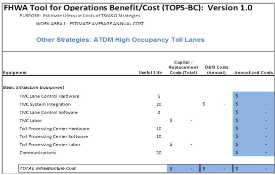 Source: FHWA TOPS-BC Figure 35. Screenshot. Tool for Operations Benefit-Cost Analysis Advanced Transportation Demand Management High Occupancy Toll Lanes Costs Page (part 1). 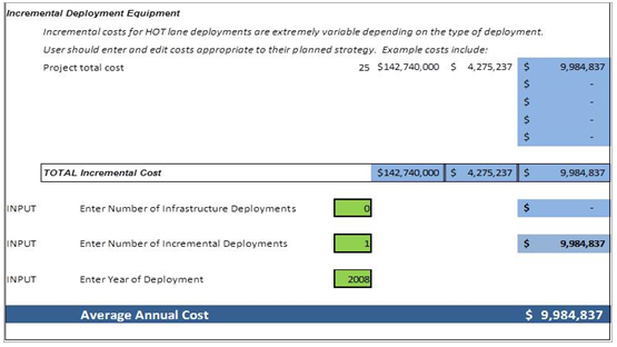 Source: FHWA TOPS-BC Figure 36. Screenshot. Tool for Operations Benefit-Cost Analysis Advanced Transportation Demand Management High Occupancy Toll Lanes Costs Page (part 2). BenefitsThe steps for the benefits calculations are described for the southbound direction. The step for the northbound direction must use a separate TOPS-BC spreadsheet template, but they are identical. Refer to the benefits assumptions described above.
The spreadsheet immediately calculates the Total Average Annual Benefit. All of these steps are repeated for the northbound TOPS-BC spreadsheet using the appropriate northbound volumes and speeds. All of the green boxes may be used to enter additional local data if they are available. In this case study, there may have been crash data and value of time data available by conducting extensive analysis. However, previous studies have indicated that local data does not usually vary significantly from the national default data and it was decided that the effort to obtain local data for crashes and time value was not worthwhile. Additionally there is a need for data collected over a long period of time, especially for injuries and fatalities, since a small sample can skew the results. See Figures 37 and 38 for screenshots of the benefits page for the southbound direction in this case study. 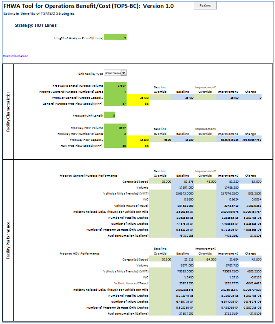 Source: FHWA TOPS-BC Figure 37. Screenshot. Tool for Operations Benefit-Cost Analysis Advanced Transportation Demand Management High Occupancy Toll Lanes Benefits Page (part 1). 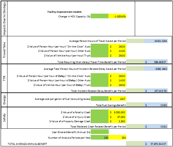 Source: FHWA TOPS-BC Figure 38. Screenshot. Tool for Operations Benefit-Cost Analysis Advanced Transportation Demand Management High Occupancy Toll Lanes Benefits Page (part 2). Preliminary Benefit Cost EvaluationBased on the northbound and southbound benefits and costs calculations using the TOPS-BC spreadsheet, the results are shown in Table 44.
Source: FHWA TOPS-BC
The large difference between the AM and PM peak numbers is due to the AM SB direction experiencing greater congestion (slower congested speed) than the PM NB peak period. Key ObservationsAfter conducting this case study and other TOPS-BC case studies and applications, several "lessons learned" have been identified. There are also a few hints to setting up the spreadsheet that will help TOPS-BC users achieve better results.
| |||||||||||||||||||||||||||||||||||||||||||||||||||||||||||||||||||||||||||||||||||||||||||||||||||||||||||||||||||||||||||||||||||||||||||||||||||||||||||||||||||||||||||||||||||||||||||||||||||||||||||||||||||||||||||||||||||||||||||||||||||||||||||||||||||||||||||||||||||||||||||||||||||||||||||||||||||||||||||||||||||||||||||||||||||||||||||||||||||||||||||||||||||||||||||||||||||||||||||||||||||||||||||||||||||||||||||||||||||||||||||||||||||||||||||||||||||||||||||||
|
United States Department of Transportation - Federal Highway Administration |
||