Transportation Systems Management and Operations Benefit-Cost Analysis CompendiumCHAPTER 5. ARTERIAL OPERATIONS
Case Study 5.1 – Hypothetical Preset Arterial Signal Coordination
Note: Chapters 2, 3, and 4 of this Compendium contain a discussion of the fundamentals of benefit-cost analyses (BCA) and an introduction to BCA modeling tools. These sections also contain additional BCA references. Project Technology or StrategyArterial signal coordination involves the coordination of traffic signal timing patterns and algorithms to smooth traffic flows—reducing stops and delays and improving travel times. Agencies can implement this strategy on a small corridor, a limited grid, or region-wide. The sophistication of the timing coordination can also vary from simple preset timing programs to more advanced traffic actuated corridor systems, to fully centrally controlled applications. Program and Project Goals and ObjectivesSince 1989, Denver Regional Council of Governments' (DRCOG) Traffic Operations Program has been working with the Colorado Department of Transportation and local governments to coordinate traffic signals on major roadways in the region. DRCOG designed the program to reduce traffic congestion and improve air quality. DRCOG was one of the first metropolitan planning organizations (MPO) to conduct such a program, and remains the leader among the very few MPOs throughout the United States involved in traffic signalization efforts. Table 8 provides a snapshot of DRCOG's 2012 annual benefits summary of projects. Links for each project provide signal timing briefs (individual benefits summary reports for each project). To view the data shown in Table 8, visit https://drcog.org/sites/drcog/files/2013%20Traffic%20Operations%20Program%20projects.pdf.
[1] Fuel @ $3.51/gal., time value @ $21.43/hr.
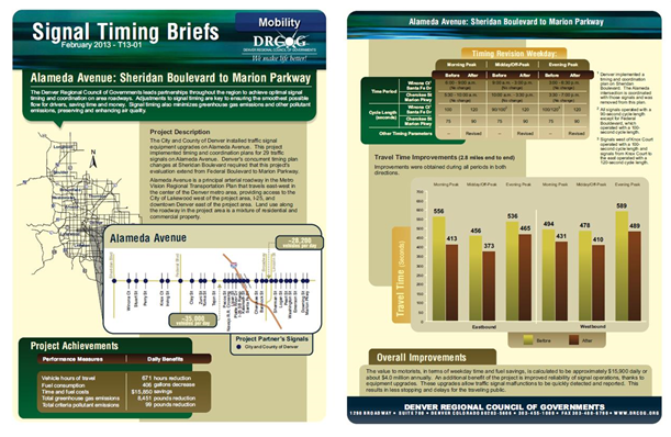
Source: DRCOG DataDRCOG collects data prior to and after deployment of signal timing to evaluate benefits. Figure 12 provides data for Alameda Avenue, the first 2013 project listed in Table 8. Visit http://www.drcog.org/documents/T13-01_Signal_Timing_Briefs_AlamedaAve.pdf for a full sized version of the flyer. Data collected include vehicles per day, length of the corridor, travel time in both directions for three time-periods (morning peak, midday/off-peak, evening peak) both before and after implementation, number of signals affected, and timing revisions. The signal timing briefs also provide estimates of daily benefits for five performance measures including vehicle hours of travel, fuel consumption, time and fuel costs, total greenhouse gas emissions, and total criteria pollutant emissions. According to the Alameda Avenue Signal Timing Brief, "Adjustments to signal timing are key to ensuring the smoothest possible flow for drivers, saving time and money. Signal timing also minimizes greenhouse gas emissions and other pollutant emissions, preserving and enhancing air quality." Benefit Cost EvaluationState DOTs, MPOs and other local transportation agencies can use benefit cost evaluation to determine whether to implement traffic signal timing programs and projects. Benefit-cost analysis can inform decision-makers as to where the best locations to improve signal timing and the most cost-effective alternatives to employ. There is a variety of pre-developed tools available to conduct benefit cost evaluation. Users can also conduct benefit-cost analysis using their own custom spreadsheets or models. TOPS-BC, an FHWA developed spreadsheet-based tool, is one option. TOPS-BC also has a function designed to aid users in identifying additional tools. The following presents the methodology and results of using TOPS-BC for a deployment of preset signal timing. While based on actual deployment information, this case study produces hypothetical results. The purpose of this example is to highlight how TOPS-BC can be deployed to evaluate similar strategies. TOPS-BC Data InputsTOPS-BC provides input defaults for most variables that a planner would use in the evaluation of a signal-timing project. If a planner was looking at a system similar to this signal-timing project example, he could use the TOPS-BC defaults, or generate new data to make the example as realistic as possible by applying local data, which the TOPS-BC user can apply in place of the defaults. This also allows the TOPS-BC user to test the impact of changes in selected input data. For example, the TOPS-BC user can perform the analysis for examples that highlight local or recent information for their project using different technology costs, traffic levels, wait times, etc. Table 9 provides a listing of the required input cost variables to run TOPS-BC for a preset traffic signal coordination project. TOPS-BC supplies many of the required inputs to run the model as shown in the final column of Table 9. The user must supply inputs that TOPS-BC does not provide. Each of the items shown in the final column of Table 9 are included in the default input data set, but may be replaced with user supplied data as shown. If the TOPS-BC user enters user-supplied data, it will override the default value and TOPS-BC will use that data in all calculations that call for that input data.
1 Capacity is calculated as 4 lanes for 3 hours at 2250 v/l/h. Lane capacities per hour from the Highway Capacity Manual (HCM).
Note: For a detailed discussion of TOPS-BC data input procedures and options, see the TOPS-BC Manual at: http://plan4operations.dot.gov/topsbctool/index.htm Model Run ResultsTable 10 summarizes the benefits and costs that TOPS-BC calculated. The table shows total annual costs of $218,571. Additional detail in the TOPS-BC model provides information on costs by year as well as total net present value costs. According to TOPS-BC, the first year costs were $404,550 with continuing annual cost for the 20-year analysis period of $201,550. This results in a 20-year net present value of just over $1.76 million.
Since the deployment on Alameda Avenue is already complete, the local agency could enter the actual cost experience. TOPS-BC provides some cost defaults, but users are encouraged to review these values and make changes based on local data. Users may also wish to disaggregate costs by lower level traffic signal subsystem as was done in Case Study 5-2. Benefits TOPS-BC estimates benefits from the preset signal timing deployment from travel time savings, change in travel time reliability, reduced energy consumption and reduced crash events. Together they result in annual benefits of about $1.5 million. These benefits are in the range of benefits shown in Table 10 which range from $600 thousand to $6.2 million per project. In this case, TOPS-BC estimates that the project benefits far exceed the costs by a ratio of 7 to 1. This positive result accrues from a gain in operating efficiency for the arterial system reducing travel time and fuel consumption. Prior to introducing the arterial signal coordination, insufficient capacity during the morning and evening peak traffic periods led to congestion and lost time for road users. With the introduction of improved traffic signal timing, traffic flows were smoother reducing stops and delays, and improving travel times. TOPS-BC also estimated a substantial reduction in energy (fuel consumption) costs due to congestion relief. The number of crashes was also estimated to decline slightly, providing an added cost reduction benefit. Key ObservationsThis case examines how users can employ TOPS-BC to evaluate the benefits and costs of a traffic signal coordination project. Colorado's Alameda Avenue project provides some of the data to illustrate how a user can run TOPS-BC. By conducting post deployment BCA, DRCOG and CDOT built up a data base of signal control costs and benefits that could inform the decision process for future deployment consideration. Case Study 5.2 – Adaptive Traffic Signal Control in Greeley and Woodland Park, Colorado
Note: Chapters 2, 3, and 4 of this Compendium contain a discussion of the fundamentals of benefit-cost analyses (BCA) and an introduction to BCA modeling tools. These sections also contain additional BCA references. Project Technology or StrategyAdaptive signal control systems coordinate control of traffic signals across a signal network, adjusting the lengths of signal phases and other parameters based on prevailing traffic conditions. This innovative technology uses real-time data collected by system detectors to optimize signal timing for each intersection in the corridor. The use of real-time data means that signal timing along the corridor changes to accommodate the traffic patterns at any given time of the day. There are many different adaptive traffic signal control systems. Project Goals and ObjectivesThe City of Greeley implemented adaptive traffic signal control systems on 10th Street (US 34 Business) in Greeley and US 24 in Woodland Park. The Colorado DOT (CDOT) selected two alternative systems, System A and System B, for implementation. CDOT commissioned a study to summarize the evaluation results of the two systems. The purpose of the study was to summarize the results of the evaluation conducted regarding the implementation of two different adaptive traffic signal control systems in Colorado: the System A system on 10th Street (US 34 Business) in Greeley and the System B on US 24 in Woodland Park. The intent of the evaluation was not to make a recommendation for a specific system, but to report a comparison of the two systems, the requirements for installation and operations, and the benefits obtained from each system. This would allow decision makers and others interested in this innovative technology to make informed decisions regarding the installation of such a system on other highways and roadways within their jurisdictions DataThe study collected data on before and after conditions and costs in order to conduct a benefit-cost analysis. Before and After Conditions The study evaluated corridor operations for both before and after conditions. Table 11 shows the results of the before and after travel time runs for the two corridors for both weekday and weekend traffic conditions. The percentages represent the combined improvement for travel times for a total of six runs through the corridor in each direction of travel during six time-periods for a weekday and one time-period for the weekends.
Source: Colorado DOT
Installation Costs The study also calculated the actual costs that the agencies had to spend to install the new systems. Table 12 shows the costs associated with the installation of the systems, based on information provided by each agency. Implementing the System A adaptive control system on 10th Street cost approximately $905,500, while the System B system cost about $176,300. Both of the systems installed required the agencies to spend additional funds to upgrade the existing signal system equipment in order to accommodate new system or operational needs. On 10th Street, several of the existing controller cabinets were not large enough to accommodate the new equipment and some of the intersections were in need of a new conduit to accommodate the wiring of new video detection cameras and their associated repeater devices. In addition, the installation required a communication system in order to ensure the controllers at each intersection could communicate with each other. It is possible that a corridor could have System A installed without the need to spend funds on any improvements, which would have saved almost $500,000 of the total $905,000 spent to install the system. On US 24, approximately $13,100 of the system installation costs was for new controllers to ensure the ability to run the firmware necessary to operate System B. Again, it is possible that this expense would not be necessary on another corridor, which would have reduced the overall cost of the project.
The study included additional analysis to compare how much would have been spent maintaining and retiming the existing signal systems compared to how much the agencies expected to spend maintaining the new systems. One main assumption for maintaining the existing systems is the need to retime the signals every five years or approximately four times in the next 20 years. Benefit Cost EvaluationThe benefit-cost analysis determined the payback period for each system, as well as the benefits that CDOT, the City of Greeley, but more importantly the general public and roadway users would realize in the future. Table 13 provides the factors the study used to calculate benefits and costs.
The local agencies directly provided the cost data. The following sections describe the calculation of each of the benefit categories. Calculation of Benefits Travel Time: The analysis multiplied total travel time (vehicle-hours) by the value of time and vehicle occupancy values for the area to calculate the cost savings in terms of reduced travel time. Fuel Consumption: The analysis multiplied total travel time (vehicle-hours) by fuel consumption rates and the average per gallon fuel cost for the area. Side-Street Delay: The analysis used the Highway Capacity Manual method for field measurement of intersection control delay to calculate intersection control delay and LOS. Travel Time. The value of travel time is calculated as: Figure 13. Equation. The Value of Travel Time. Where: ΔTT is the change in Travel Time The value of time for both corridors was obtained from research performed by FHWA and input from the CDOT Division of Transportation Development (DTD) staff and was found to be $15.00 per person per hour. CDOT staff indicated a recent study for the area identified the average vehicle occupancy for both of the highways is 1.3 people per vehicle. Annual costs and benefits were computed based upon a 350 day year (250 weekdays and 100 weekend days) to best capture the majority of typical traffic volume days. The remaining days of the year were considered non-typical travel days (holidays, events, weather, etc.) and were omitted from the computation. Fuel Consumption. Fuel consumption is calculated as: Total Travel Time (vehicle-hours)* Fuel Consumption Rate * Average Price Internet research identified average fuel costs of $3.65 per gallon in the Greeley area and $3.50 in the Woodland Park area. Current fleet average fuel consumption rates at various speeds are available from EPA. Side-Street Delay. For a signal control project with fixed cycle lengths during specific periods of the day, traffic simulation software can estimate side-street delay at study intersections. Because the adaptive traffic signal systems are continuously changing signal timing parameters to react to real-time travel demand, the analysis used the Highway Capacity Manual method for field measurement of intersection control delay to calculate intersection control delay and level of service (LOS). Video recordings were conducted at four intersections on each corridor, as identified by agency staff, to capture the before and after conditions during the morning, midday, and evening weekday peaks. Summary of BenefitsTable 14 provides the benefits of implementing the adaptive signal control systems. The systems result in significant savings to both corridors, with 10th Street experiencing a predicted annual user savings of more than $1.326 million dollars per year and US 24 users experiencing an annual savings of almost $900,000 per year.
1 Assumes benefits realized for 350 days.
Source: Colorado DOT Model Run ResultsA consultant, using a standalone custom in-house analysis, conducted the benefit-cost analysis. Table 15 provides various metrics of benefits, costs, and savings that the consultant team calculated. Overall, benefit-cost ratios vary from 1.58 to 6.10 for the first year that the systems are in operation. Based on the analysis, Region 4 and the City of Greeley will accrue benefits of approximately $8.9 million over the first 20 years with System A managing the traffic operations on the 10th Street corridor. At the same time, Region 2 will accrue benefits of about $5.8 million over the first 20 years with System B managing the traffic operations on the US 24 corridor.
Note: Actual projects had unusual costs; minimal project represents the expected costs for other projects.
Source: Colorado DOT Key ObservationsThis case evaluates the introduction of adaptive traffic signal control systems on two arterials. Adaptive signal control systems coordinate traffic signals across a network, adjusting the signal timing parameters based on prevailing traffic conditions. Prior to and after the deployment, the study collected data on performance to be able to compare the changes brought about by the deployment. The data collection revealed improvements in terms of travel time, fuel consumption and side street delay. The study also collected data on implementation costs and estimated implementation cost savings for specific costs that would not be necessary on another corridor. The analysis illustrates how benefit-cost analysis can be used to compare alternative adaptive traffic signal systems. It also informs decision makers and others interested in this innovative technology to make informed choices regarding the installation of such a system on other highways and roadways within their jurisdictions. Case Study 5.3 – Adaptive Traffic Signal Control
Note: Chapters 2, 3, and 4 of this Compendium contain a discussion of the fundamentals of benefit-cost analyses (BCA) and an introduction to BCA modeling tools. These sections also contain additional BCA references. Project Technology or StrategyAdaptive signal control systems coordinate control of traffic signals across a signal network, adjusting the lengths of signal phases based on prevailing traffic conditions. This innovative technology uses real-time data collected by system detectors to optimize signal timing for each intersection in the corridor. The use of real-time data means that signal timing along the corridor changes to accommodate the traffic patterns at any given time of the day. Project Goals and ObjectivesA State DOT commissioned the evaluation of an adaptive traffic signal control system on a principal arterial. The goal of the traffic signal control project was to reduce congestion, smooth traffic flows, improve travel times, maximize the benefits of signal timing, and potentially reduce crashes, which delay the need for more costly improvements such as adding capacity to the corridor. The corridor primarily serves local traffic, including commuters, during the week and visitors and recreational travelers on the weekends. The traffic patterns can vary rapidly and unpredictably on the weekend due to the nature of recreational travelers and weather conditions that may cause travelers to change when they begin and terminate their recreational activities. Thus, the current application of time-of-day based signal coordination plan were identified as inadequately adjusting to the travel patterns of the visitors that come to and pass through the area. DataThe commissioned report described the changes that were required to install and operate the adaptive signal control system, including costs for installation and maintenance, and provide a comparison of before and after implementation measures of effectiveness (MOE) to quantify the benefits to traffic operations within the study area. The study collected data on before and after conditions and costs in order to conduct a benefit-cost analysis. Before and After Conditions. The study evaluated corridor operations for both before and after conditions. The study evaluated the following MOEs for the corridor:
Calculation of Benefits Travel Time: The analysis multiplied total travel time (vehicle-hours) by the value of time and vehicle occupancy values for the area to calculate the cost savings in terms of reduced travel time. Fuel Consumption: The analysis multiplied total travel time (vehicle-hours) by fuel consumption rates and the average per gallon fuel cost for the area. Side-Street Delay: The analysis used the Highway Capacity Manual method for field measurement of intersection control delay to calculate intersection control delay and LOS. Installation Costs. The study calculated the actual costs that the agencies had to spend to install the new systems. The study also conducted additional analysis to compare how much would have to be spent maintaining and retiming the existing signal systems compared to how much the agencies expected to spend maintaining the new systems. One main assumption for maintaining the existing systems was the need to retime the signals every five years or approximately four times in the next 20 years. Benefit Cost EvaluationThe purpose of the benefit cost evaluation was to summarize the results of the evaluation conducted regarding the implementation of the adaptive traffic signal control system. Approach. The benefit-cost analysis determined the payback period for each system, as well as the benefits that the State DOT and local agencies, and more importantly the general public and roadway users, would realize in the future. Table 16 provides the factors the study used to calculate benefits and costs.
The local agencies directly provided the cost data. The following sections describe the calculation of each of the benefit categories. Travel Time. The analysis multiplied total travel time (vehicle-hours) by the value of time and vehicle occupancy values for the area to calculate the cost savings in terms of reduced travel time. The study obtained the value of time from research performed by FHWA and input from the State DOT staff and was found to be $15.00 per person per hour. A recent study for the area identified the average vehicle occupancy for the highway was 1.3 people per vehicle. Annual costs and benefits were computed based upon a 350 day year (250 weekdays and 100 weekend days) to best capture the majority of typical traffic volume days. Fuel Consumption. The analysis multiplied total travel time (vehicle-hours) by fuel consumption rates and the average per gallon fuel cost for the area. Internet research identified average fuel costs. Side-Street Delay. For a signal-timing project with fixed cycle lengths during specific periods of the day, traffic simulation software can estimate side-street delay at study intersections. Because the adaptive traffic signal systems are constantly changing cycle lengths to react to real-time travel demand, the analysis used the Highway Capacity Manual method for field measurement of intersection control delay to calculate intersection control delay and LOS. Video recordings were conducted at four intersections, to capture the before and after conditions during the morning, midday, and evening weekday peaks. Model Run ResultsA consultant, using a standalone custom in-house analysis, conducted the benefit-cost analysis. The consultant reported that, based on the benefits and cost to install the new system, the system implementation will:
Table 17 provides a summary of the results of the benefit-cost analysis.
Key ObservationsThis case identifies the evaluation of an adaptive traffic signal control systems on an arterial. Adaptive signal control systems coordinate control of traffic signals across a signal network, adjusting the lengths of signal phases based on prevailing traffic conditions. Prior to and after the deployment, the study collected data on performance to be able to compare the changes brought about by the deployment. The data collection revealed improvements in terms of travel time, fuel consumption and side street delay. The study also collected data on implementation costs and conducted a benefit-cost analysis. The benefit-cost analysis did not properly frame the costs and benefits in relation to the alternatives and did not incorporate net present values of the streams of benefits and costs over the project life. The analysis illustrates how the use of a model such as TOPS-BC can structure the analysis to insure the analysis avoids common mistakes and produces meaningful results. Case Study 5.4 – Hypothetical Roundabouts
Note: Chapters 2, 3, and 4 of this Compendium contain a discussion of the fundamentals of benefit-cost analyses (BCA) and an introduction to BCA modeling tools. These sections also contain additional BCA references. Project Technology or StrategyModern roundabouts are a type of intersection characterized by a generally circular shape, yield control on entry, and geometric features that create a low-speed environment. Modern roundabouts provide a number of safety, operational, and other benefits when compared to other types of intersections. On projects that construct new or improved intersections, planners should examine the modern roundabout as an alternative. In the planning process for a new or improved intersection where a traffic signal is under consideration, a modern roundabout should likewise receive serious consideration as an alternative. This begins with understanding the site characteristics and determining a preliminary configuration. There are a number of locations where roundabouts are advantageous and a number of situations that may adversely affect their feasibility. As with any decision regarding intersection treatments, planners should take care to understand the particular benefits and trade-offs for each project site. Project Goals and ObjectivesThe Washington State DOT's (WSDOT) website includes a page devoted to Roundabout Benefits (http://www.wsdot.wa.gov/Safety/roundabouts/benefits.htm). On that page, WSDOT states, "Studies have shown that roundabouts are safer than traditional stop sign or signal-controlled intersections." The WSDOT webpage also notes that roundabouts reduce delay and improve traffic flow. The webpage states, "Contrary to many peoples' perceptions, roundabouts actually move traffic through an intersection more quickly, and with less congestion on approaching roads. Roundabouts promote a continuous flow of traffic. Unlike intersections with traffic signals, drivers don't have to wait for a green light at a roundabout to get through the intersection. Traffic is not required to stop – only yield – so the intersection can handle more traffic in the same amount of time." Finally, the WSDOT webpage also notes that roundabouts are less expensive than traffic signals. The webpage states, "The cost difference between building a roundabout and a traffic signal is comparable. Where long-term costs are considered, roundabouts eliminate hardware, maintenance and electrical costs associated with traffic signals, which can cost between $5,000 and $10,000 per year." Given these advantages, planners and traffic engineers may want to estimate the benefits of conversion of a signalized intersection to a roundabout. These practitioners can readily use TOPS-BC to perform such calculations at the sketch planning level. Data
Note: The data used in this Case Study is used for illustrative purposes and not intended to suggest expected performance benefits from roundabouts. The next Case, Case 5-5, shows different operational and safety performance data assumed in Maryland.
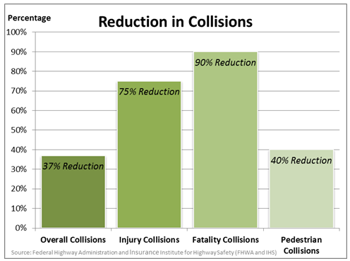
The WSDOT webpage cites a study by the Insurance Institute for Highway Safety (IIHS) that estimates that roundabouts reduced injury crashes by 75 percent at intersections that achieved traffic control through stop signs or signals. Figure 15, reprinted from the WSDOT webpage and based on studies by the IIHS and Federal Highway Administration, shows that roundabouts may achieve:
The WSDOT webpage cites studies by Kansas State University (http://www.ksu.edu/roundabouts/) that measured traffic flow at intersections before and after conversion to roundabouts. In each case, installing a roundabout led to a 20 percent reduction in delays. Benefit Cost EvaluationState DOTs, MPOs and other local transportation agencies can use benefit cost evaluation to aid in determining whether to implement an intersection project such as a roundabout. There is a variety of pre-developed tools available to conduct benefit cost evaluation. Users can also conduct benefit-cost analysis using their own custom spreadsheets or models. TOPS-BC, an FHWA developed spreadsheet-based tool, is one option. TOPS-BC also has a function designed to aid users in identifying additional tools. TOPS-BCTOPS-BC provides input defaults for most variables that a planner would use in the evaluation of a project. While TOPS-BC does not provide defaults for roundabouts, the user could still use TOPS-BC by adding a new strategy to the benefit estimation capability. TOPS-BC Data Inputs. This hypothetical TOPS-BC case assumes that the initial costs of adding a signalized intersection and a roundabout are comparable and is just interested in the magnitude of benefits. User-supplied Performance Data
The user has several options for creating a new strategy in TOPS-BC. These include:
This case assumes that the user has chosen the first option and will simply rename the strategy. Since the user is evaluating a roundabout, which is an arterial intersection project, the case assumes the user selected the "Arterial Strategy" "Signal Coordination." Figure 16 shows a partial view of the Signal Coordination Model sheet with the strategy renamed to "Roundabout." 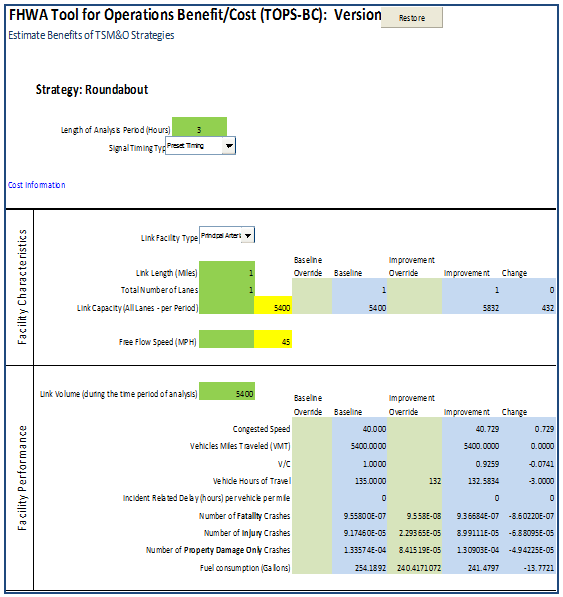 Source: Federal Highway Administration TOPS-BC
Figure 16. Screenshot. A Run for Roundabout Benefits Using the Tool for Operations Benefit-Cost Analysis. User and TOPS-BC Supplied Site Data. Entering user-supplied data allows the TOPS-BC user to make the analysis as specific as possible for their project. This case assumes the TOPS-BC user has some specific site characteristics including Length of Analysis Period (3-hour peak-period), Link Length (one-mile), and Total Number of Lanes (one lane) and Link Volume (5,400 vehicles per period). As congestion exists in both directions during the peak, this case assumes the user sets the Number of Analysis Periods per Year to 500. None of these values override the values for which TOPS-BC provides a default value, such as Link Capacity (5,400 vehicles per period) or Free Flow Speed, for which TOPS-BC provides a value of 45 miles per hour. User Supplied Performance Data. This case assumes that the TOPS-BC user enters specific data on the performance of roundabouts. TOPS-BC uses five performance characteristics in calculating the benefits. These performance characteristics, along with the user-entered values include:
Model Run ResultsTOPS-BC estimates the annual benefits of the roundabout resulting from travel time savings, change in travel time reliability, reduced energy consumption and reduced crash events. Table 18 provides each of these benefits as TOPS-BC calculates and shows them on the "My Deployments" page. Together they result in annual benefits of $76,020.
With the introduction of a roundabout, rather than a traditional signalized intersection, traffic flows are smoother, reducing stops and delays, and improving travel times. TOPS-BC estimates a substantial reduction in travel times resulting in substantial travel time benefits. This reduction in stops and delays also reduces energy (fuel consumption) costs. Due to low travel speeds (drivers slow down and yield to traffic before entering a roundabout), no light to beat (roundabouts promote a continuous circular flow of traffic), and one-way travel (roundabouts direct drivers counterclockwise and eliminate the possibility for T-bone and head-on collisions) the number of crashes also declined, providing a safety benefit due to crash cost reduction. Key ObservationsThis case examines how users can employ TOPS-BC to evaluate the benefits of a roundabout project. Washington State DOT's roundabouts webpage provides some of the data as an example of what a user might consider to run TOPS-BC. The TOPS-BC run estimates that the project would generate annual benefits of $65,204. This example illustrates how the user can add new strategies to TOPS-BC and use data from real world projects. In this case we also used information and methods contained in TOPS-BC on fuel savings from adaptive signal control projects to estimate fuel savings from roundabout installation. This is an approximation of the fuel savings from roundabouts. If consideration of roundabouts continued beyond this preliminary review, the analyst might consider developing better estimates of roundabout fuel savings. Case Study 5.5 – Effectiveness of Roundabouts in Maryland
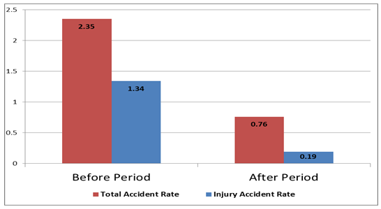
Note: Chapters 2, 3, and 4 of this Compendium contain a discussion of the fundamentals of benefit-cost analyses (BCA) and an introduction to BCA modeling tools. These sections also contain additional BCA references. Project Technology or StrategyModern roundabouts are a type of intersection characterized by a generally circular shape, yield control on entry, and geometric features that create a low-speed environment. Modern roundabouts provide a number of safety, operational, and other benefits when compared to other types of intersections. On projects that construct new or improved intersections, planners should examine the modern roundabout as an alternative. Figure 17 provides a diagram illustrating the key characteristics of a modern roundabout. 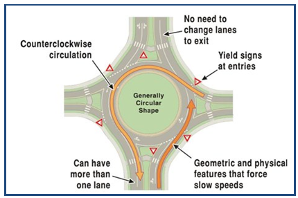 Source: Maryland DOT
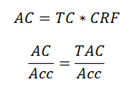
Figure 17. Diagram. Key Roundabout Characteristics. In the planning process for a new or improved intersection where a traffic signal or stop control is under consideration, a modern roundabout should likewise receive serious consideration as an alternative. This begins with understanding the site characteristics and determining a preliminary configuration. There are a number of locations where roundabouts are advantageous and a number of situations that may adversely affect their feasibility. As with any decision regarding intersection treatments, planners should take care to understand the particular benefits and trade-offs for each project site. Calculations are based on the anticipated accident experience expected to occur had no roundabouts been installed compared to the actual after period accident experience. Project Goals and ObjectivesThe State of Maryland published a report that evaluates the effectiveness of roundabouts in Maryland. Studies have found that one of the benefits of roundabout installations is the improvement of overall safety performance. The calculations in the report are based on the anticipated accident experience expected to occur had no roundabouts been installed compared to the actual accident experience at the roundabout locations. The state has found that single-lane roundabouts perform better than two-way, all-way stop and signalized intersections. Although the frequency of crashes is not always lower at roundabouts, particularly multi-lane roundabouts, injury rates are lower. DataThe Maryland analysis indicates that at the 15 locations where Maryland has installed single lane roundabouts there has been a 68 percent decrease in the total accident rate per million vehicles entering the intersection (mve). In addition, there was a 100 percent decrease in the fatal accident rate/mve, an 86 percent reduction in the injury accident rate/mve, and a 41 percent reduction in the property damage only accident rate/mve. Figure 18 provides before and after graphical comparisons of the total and injury-only accident rates. The accident data is from the Maryland State Highway Administration (MDSHA) accident database. This database consists of all accidents for which the state received an official accident report form from the Maryland Automatic Accident Reporting System (MAARS). The study collected accident data for 15 single-lane mini roundabouts. The before and after period vary depending on completion dates of the roundabouts. Maryland reports that the initial total cost of the roundabouts was $6,219,505. The state assumes the projects have a 15-year service life. The state assumes there is no before and after annual operating and maintenance cost or salvage value for these projects. Benefit Cost EvaluationThe Maryland study utilized both the cost-effectiveness and the benefit cost techniques. The cost-effectiveness method determines the cost of preventing a single accident to decide whether the project cost was justified. This technique does not price benefits. Instead, the method determines the cost of reducing accidents by severity. An alternate method is the benefit cost technique. The benefit-cost analysis compares the Annual Benefit (AB) to the Equivalent Uniform Annual Cost (EUAC) over the entire service life of the roundabouts. Maryland considers any project that has a benefit-cost ratio greater than 1.0 to be economically successful. Use of this method requires that the dollar value is placed on all cost and benefit elements related to the project. Maryland has developed its own average accident cost figures, stratified by severity. Model Run ResultsThe Maryland State Highway Administration's Traffic Safety Analysis Division, using a stand-alone custom in house analysis, conducted the cost-effectiveness analysis and benefit-cost analysis. This analysis used Maryland's own accident cost figures by severity, which reports the average cost of a fatal accident at $4,167,062, the average injury accident cost at $110,584, and average property damage only accident cost at $26,156. Maryland's objective in conducting the cost-effectiveness evaluation was to determine the amount of dollars spent to reduce one accident. Where: AC = Levelized Annual Cost for Roundabout Program in Maryland
Source: Maryland DOT
MDSHA estimated the annual benefit of crash avoidance by using the crash frequency and costs by crash type prior to the roundabout installation to estimate the expected crash frequency and costs after installation. The expected crashes without the roundabouts were compared to the actual crash results for a 4.5 year period after deployment. This resulted in an annual savings of $9.8m. For more detail on the MDOT benefit calculations, see the report referenced at the end of this case. Equivalent Uniform Annual Cost (EUAU) Equivalent Uniform Annual Cost is the "payment" required to fund the Life Cycle Cost over the service life. It is calculated as:
Where: A/P = Annualized program cost ($/sq. ft.) Unlike the cost effectiveness evaluation, which determines how many dollars the state must spend to reduce one accident, the benefit-cost analysis considers the initial cost of the projects for the entire service life (15-years) of the roundabouts. The Maryland BCA converts initial cost into an EUAC, also referred to as levelized cost. The analysis then divides the EUAC into the AB to reveal the BCR. The Maryland analysis does this to calculate the amount of money spent over the 15-year service life for roundabout installations as opposed to just calculating the dollar value realized through the annual safety benefits in accident prevention. The analysis indicates that for every dollar spent on the roundabout installation over the entire 15-year service life, the state anticipates that the roundabout users will realize approximately $15 in benefits through accident reduction. This calculation is:
Source: Maryland DOT
Key ObservationsThis case presents the results of an economic evaluation of roundabouts conducted by Maryland State Highway Administration's Traffic Safety Analysis Division, Office of Traffic & Safety. The calculations are based on the anticipated accident experience had no roundabouts been installed, compared to the actual after period accident experience. The state found that single-lane roundabouts perform better than two-way, all-way stop and signalized intersections. The state utilized both the cost-effectiveness and the benefit cost techniques. The analysis illustrates how both cost-effectiveness and benefit-cost analysis can be useful to compare alternatives to operational strategies. It informs decision makers and allows others interested in this technology to make informed choices regarding the installation of such a system on roadways within their jurisdictions. Cost-effectiveness (CE) and BCA are related and may both be appropriate ways for a decision maker to evaluate a potential deployment. For example, CE is better suited to situations when alternatives are expected to provide equal outcomes (benefits), so that the differentiator between alternatives is cost. BCA is more comprehensive, considering costs and benefits of alternative projects and project designs that may provide different levels and timing of both costs and benefits. Case Study 5.6 – Effectiveness of Arterial Management in Florida
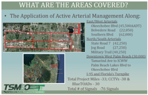
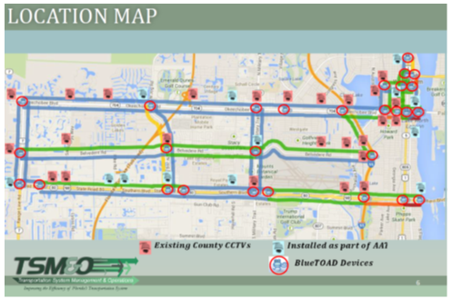
Note: Chapters 2, 3, and 4 of this Compendium contain a discussion of the fundamentals of benefit-cost analyses (BCA) and an introduction to BCA modeling tools. These sections also contain additional BCA references. Project Technology or StrategyThe following case study was prepared by Cambridge Systematics, Inc. for the Florida Department of Transportation (FDOT) as part of the "TOPS-BC Florida Guidebook" and is reproduced here with permission. FDOT District 4 in collaboration with Palm Beach County Traffic Engineering Department (PBC TED) initiated the "Living Lab" pilot project in 2012 to actively monitor, manage, and improve arterial operations along three major east-west corridors – Okeechobee Boulevard, Belvedere Road, and Southern Boulevard between SR 7 and I-95. Project Goals and ObjectivesAs part of this initiative, FDOT District 4 installed several CCTV cameras and BlueTOAD vehicle detection devices along these corridors to monitor traffic conditions and collect travel times in real-time. In addition, FDOT District 4 provided staffing resources at the Palm Beach County Traffic Management Center to monitor real-time traffic conditions, detect incidents, and support Palm Beach County Signal Timing staff in implementing real-time signal timing changes to improve traffic flow and reduce motorist delay. FDOT District 4 Freeway Intelligent Transportation Systems (ITS) staff and Palm Beach County Signal Timing Engineers work together to improve freeway-arterial coordination during incidents on I-95 in Palm Beach County. The hours of operation are Monday through Friday from 7a.m. to 7p.m. Figures 22 and 23 show the location of the Living Lab and device locations along the instrumented roadways. AssumptionsThere were many assumptions that went into the TOPS-BC analysis for the Palm Beach Living Lab case study. Also, several limitations should be noted. These are listed in the following sections. Costs Costs for implementing and operating the Living Lab project were provided by the PBC TED. The cost of equipment and devices installed in the study area (along with operations and maintenance costs) were assigned to the Incremental Deployment cost. Several costs were also provided by PBC TED that are used to manage the entire countywide traffic control system, i.e. TMC operators, incident management software, ATMS.now license, and INRIX data subscription. These costs were assigned to the basic infrastructure costs because they are needed to operate the countywide traffic signal system with or without the Living Lab project. Benefits It is not possible to analyze more than one corridor at a time using TOPS-BC. For this case study, a separate TOPS-BC spreadsheet was set up for each of the six primary corridors in the study area. A process to determine an overall BC ratio for the Living Lab program is described later in this section. Link volume data was obtained from intersection counts conducted periodically by the PBC TED. The volumes are part of a countywide traffic count program and were counted on a rotating basis between 2010 and 2013. The link volume used in the calculation was determined by averaging the approach volumes of each intersection available in the intersection count program for the corridor (considering the east/west approaches on Okeechobee, Belvedere and Southern and the north/south approaches on Military, Jog and SR 7) and using the highest average volume as the volume in the spreadsheet. An example of the volumes for Okeechobee Blvd. is shown in Table 21. The volumes in the count program are defined by approach, EA is the east approach or westbound. The peak volume is the p.m. peak hour in the east approach (westbound).
Source: Florida DOT
EA= east approach • NA = north approach • SA = south approach • WA = west approach The highest total volume is the sum of the east approaches. The average peak approach one hour volume is 2552. Each of the other corridor volume inputs was determined in this manner. Speeds were also obtained from the PBC TED. The FDOT Systems Planning Office standard for free flow speed is the speed limit plus 5 miles per hour (mph). The speed limit varies in sections of the corridors between 35 and 50 mph. The free flow speed should then be between 40 and 55 mph. In this case study PBC TED provided data that allowed the free flow speed to be determined by averaging off-peak travel times along each corridor using the Bluetooth detectors and calculating the average speed over several months. The baseline speed is based on historic travel time data collected prior to the implementation of the Living Lab project. The Baseline Override speed shown is the speed for the peak hour and direction of the highest volume, in the Okeechobee case above the speed used in the spreadsheet is for the PM EA approach. The Improvement Override speed was collected after implementation of the Living Lab project by PBC TED using the Bluetooth detectors and reported in the PBC TMC Active Arterial Management Program Performance Measures Monthly Report. The speeds used were from the November 2013 report. The number of analysis periods is different from for the I-95 Express Lanes case study. The benefits are accrued for the peak hour in the peak direction, which is represented by 250 analysis periods, which are the average number of work days in a year (total days minus weekends and holidays). However, while the p.m. peak hour was found to have the highest volumes, significant benefits are also accrued for the a.m. peak hour. In a case where the a.m. peak hour has the highest volumes, the p.m. peak hour should be included in the same manner. In order to account for those benefits the peak volume in the a.m. peak period was identified and a ratio of that volume to the highest peak hour volume was determined. That portion of the 250 analysis periods was added to the 250 original analysis periods. (Another option is to conduct two separate BCA analyses, one for each direction.) Using the Okeechobee example in Table 21, the corresponding peak period is the a.m. peak hour. The east approach was the highest volume approach in the a.m. period so that volume (2153) was used. The a.m. peak to p.m. peak hour volume ratio is 2153/2552 or 0.844. The a.m. peak should account for 84.4 percent of the amount of analysis periods that the p.m. peak hour provides, so 250 X .844 is 211; 211 + 250 is 461. The amount of benefits accrued in both the a.m. and p.m. peak hours is accounted for by using 461 analysis periods. The other corridors' benefits were calculated in the same manner. This methodology provides a conservative estimate of benefits since only two peak hours of benefits are accounted. Volumes for periods other than the peak hour were not available. National average (default) input data was used for crashes, fuel consumption, and the value of time. This was due to the difficulty in collecting and summarizing data or the fact that data were not available at all. Limitations. While TOPS-BC does include the benefits due to time savings in recurring and non-recurring travel during each analysis period, the impacts of improvements due to improved travel time reliability are included only in freeway analysis. Reliability has been recognized as an important consideration to travelers. Improving reliability is a benefit to travelers. The SHRP 2 research project dedicated a significant portion of its resources to defining, understanding and measuring reliability. SHRP 2 has released several reports relating to the topic. Not all of this research has been added to the TOPS-BC model Version 1. TOPS-BC V1 now estimates only the benefits from reducing incident related delay. In the future, TOPS-BC will add new code to address the current reliability benefits and add these benefits to the full BCA. The latest model will be available on the FHWA Planning for Operations web site (https://ops.fhwa.dot.gov/plan4ops/index.htm). TOPS-BC does not have a trip assignment or mode choice module, therefore the operations strategy analysis only accounts for the number of trips given for each corridor, there are no trip diversions or mode changes due to congestion. TOPS-BC will provide conservative estimates of benefits because only the benefits accrued during the selected time period are calculated. In many cases, additional benefits may be produced in off-peak times that are not included. Changes in air quality due the operations strategies are not accounted for in TOPS-BC. MethodologyThe following are the steps to enter input data for the Palm Beach Living Lab case study. Note that separate TOPS-BC calculations are required for each of the six corridors in the study area. The steps are the same for each corridor but the input volumes and speeds are different. Costs.
See Figure 24 for a screenshot of the Costs page for the Okeechobee Blvd. corridor in this case study. 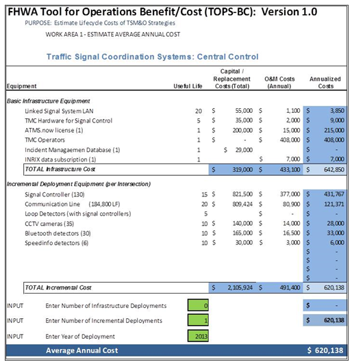 Source: FHWA TOPS-BC Figure 24. Screenshot. Tool for Operations Benefit-Cost Analysis Traffic Signal Coordination Systems Costs Page. Benefits. The Okeechobee Blvd corridor will be used as an example for providing input data to the spreadsheet.
See Figures 25 and 26 for screenshots of the Benefits page for the Okeechobee Blvd. corridor in this case study. 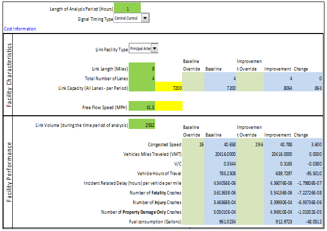 Source: FHWA TOPS-BC Figure 25. Screenshot. Tool for Operations Benefit-Cost Analysis Traffic Signal Coordination Systems Benefits Page (part 1). 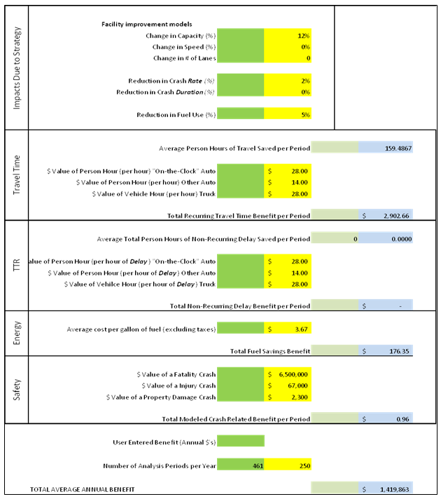 Source: FHWA TOPS-BC Figure 26. Screenshot. Tool for Operations Benefit-Cost Analysis Traffic Signal Coordination Systems Benefits Page (part 2). Preliminary Benefit Cost EvaluationBased on the six corridors benefits and costs calculations using the TOPS-BC spreadsheet, the results are shown in Table 22.
Source: Florida DOT
B/C = benefit/cost Key ObservationsAfter conducting these and other TOPS-BC case studies and applications, several "lessons learned" have been identified. There are also a few hints to setting up the spreadsheet that will help TOPS-BC users achieve better results.
| |||||||||||||||||||||||||||||||||||||||||||||||||||||||||||||||||||||||||||||||||||||||||||||||||||||||||||||||||||||||||||||||||||||||||||||||||||||||||||||||||||||||||||||||||||||||||||||||||||||||||||||||||||||||||||||||||||||||||||||||||||||||||||||||||||||||||||||||||||||||||||||||||||||||||||||||||||||||||||||||||||||||||||||||||||||||||||||||||||||||||||||||||||||||||||||||||||||||||||||||||||||||||||||||||||||||||||||||||||||||||||||||||||||||||||||||||||||||||||||||||||||||||||||||||||||||||||||||||||||||||||||||||||||||||||||||||||||||||||||||||||||||||||||||||||||||||||||||||||||||||||||||||||||||||||||||||||||||||||||||||||||||||||||||||||||||||||||||||||||||||||||||||||||||||||||||||||||||||||||||||||||||||||||||||||||||||||||||||||||||||||||||||||||||||||||||||||||||||||||||||||||||||||||
|
United States Department of Transportation - Federal Highway Administration |
||