Travel and Emissions Impacts of Highway Operations Strategies

Chapter 5. Short-Term Emissions Impacts of Operations Strategies

Overview

One of the motivations for conducting this project was to determine the effect that operations strategies have on emissions. That is, how will changes in traffic flow effected by operations result in changes in emissions. Traditionally, the impact of transportation improvements on emissions have been linked via changes in average speed. However, because the effect of operations strategies may more to smooth traffic flow in breakdown and near-breakdown conditions than to change overall speed greatly, this approach has been criticized.

The need to model emissions at a more detailed level has led to the development of emissions models based on vehicle activity (i.e., modal emissions models); see Chapter 2.0 for a discussion of these models. These models are capable of using second-by-second speed and acceleration activity from individual vehicles, also known as vehicle trajectories, as input. Vehicle trajectories can be measured in the field using specialized equipment, but for forecasting, microscopic traffic simulation models can provide them.

Integration of traffic and emissions models is still in the formative stages. As far back as the early 1990s, such integration had been accomplished for the first generation of microscopic traffic simulation models, FRESIM and NETSIM, developed and supported by FHWA. In these models, a series of lookup tables were used to estimate emissions (carbon monoxide, nitrous oxides, and hydrocarbons) and fuel consumption. The tables were defined by instantaneous speeds and accelerations and were accessed every second for every vehicle; the data were based on testing a very limited sample of vehicles conducted in the mid-1980s. Thus, total emissions and fuel consumption were built up from the lowest level possible. However, subsequent research has shown that vehicle emission production is a more complex process involving factors beyond speed and acceleration, including engine load, engine characteristics, and other factors, so the simple lookup table approach has been abandoned.

One of the first efforts to link modal emissions and microscopic traffic simulation models was the Comprehensive Modal Emissions Model (CMEM) developed under NCHRP Project 25-11. (Barth, Matthew et al., Development of a Comprehensive Modal Emissions Model, Web-Only Document 122, Transportation Research Board, April 2000) Figure 32 shows the CMEM’s link-level fuel consumption modeling methodology. Subsequently, other modal emissions models, including MOVES, have been used in conjunction with simulation models. A few examples include:

• CMEM has developed a plug-in to the Paramics microsimulation model, which calculates emission data for every vehicle in a Paramics simulation at every second. (University of California Riverside Center for Environmental Research and Technology CMEM – Comprehensive Modal Emissions Model.)
• SHRP 2 Project C10B developed a direct connection between the DynusT mesoscopic simulation model and MOVES.
• FHWA’s, Advances in Project-Level Emissions Analyses, linked the Transmodeler microscopic simulation model with MOVES. (E.H. Pechan and Associates et al., “Advances in Project Level Analyses,” prepared for FHWA, Contract No. DTFH61-10-C-0006, November 4, 2010.)

Figure 32. Graph. CMEM’s link-level fuel consumption modeling methodology.

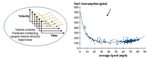
(Source: Scoara, George and Barth, Matt, CMEM User’s Guide, Version 3.01, University of California, Riverside Center for Environmental Research and Technology, June 2006.)

For this project, it was decided to use a microscopic simulation that already been calibrated and used to analyze operational strategies in conjunction with the MOVES model. Details are provided below.

Study Design

Area Studied

The simulation model that was previously used to assess the benefits of Integrated Corridor Management (ICM) in the Interstate-15 (I-15) corridor in San Diego, California was selected (microscopic formulation of the TransModeler software). (Cambridge Systematics, “Integrated Corridor Management: Analysis, Modeling, and Simulation for the I-15 Corridor in San Diego, California,”“ prepared for FHWA, December 2011.) The I-15 corridor site in San Diego, California extends from the interchange with State Road (SR) 163 in the south to the interchange with SR 78 in the north, a freeway stretch of approximately 20 miles. Also included in the study area are the following roadways:

• Centre City Parkway.
• Pomerado Road.
• Rancho Bernardo Road.
• Camino Del Norte Road.
• Ted Williams Parkway.
• Black Mountain Road.
• Scripps Parkway.

Figure 33 illustrates the Pioneer Corridor and the roadways included in the study area. I-15 is an 8- to 10-lane freeway section in San Diego providing an important connection between San Diego and cities like Poway, Mira Mesa, and Escondido, and destinations to the northeast. Figure 34 indicates the geographic location of the corridor along with the extents of the mainline study area.

The current operations on I-15 include two center-median lanes that run along eight miles of I-15 between SR 163 in south and Ted William Pkwy (SR 56) in the north. These center-median lanes are reversible high-occupancy vehicle (HOV) lanes that operate in the southbound direction in the AM peak period and in the northbound direction during the PM peak period. The current operations also allow single occupancy vehicles (SOV) to utilize the roadway for a price, thereby operating as high-occupancy toll (HOT) lanes.

The I-15 corridor is one of three primary north-south transportation corridors in San Diego County, and is the primary north-south highway in inland San Diego County, serving local, regional, and interregional travel. The corridor is a heavily utilized regional commuter route, connecting communities in northern San Diego County with major regional employment centers. The corridor is situated within a major interregional goods movement corridor, connecting Mexico with Riverside and San Bernardino counties, as well as Las Vegas, Nevada.

Modeling Approach

The microscopic component of TransModeler was utilized for the analysis of the corridor. This model also was used to evaluate the response of drivers in incident situations when they are faced with high levels of congestion. When a driver’s path choice is reevaluated, the path costs (e.g., segment travel times) are reconsidered. For driver groups defined in the model parameters as having access to real-time travel information (i.e., informed drivers), an updated travel timetable was used to evaluate path costs. Drivers belonging to a driver group that do not have access to real-time information will reconsider their paths using the same (i.e., historical) travel time information used to evaluate their pretrip paths.

Figure 33. Map. Study area I-15 corridor in San Diego, California.

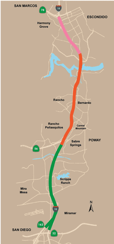
(Source: Cambridge Systematics, Inc.)

Figure 34. Map. Location and geographic boundaries of corridor.

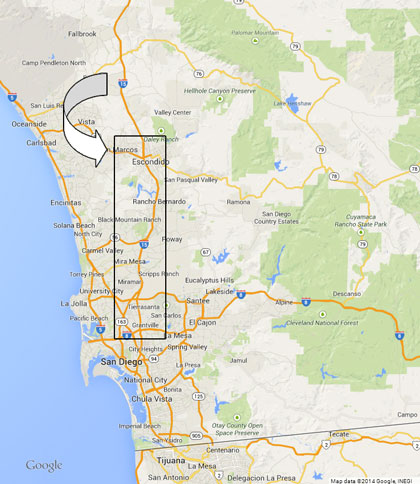
(Source: Cambridge Systematics, Inc., ©2014 Google, INEGI.)

The traffic assignment models within TransModeler allow the use of static and dynamic assignment procedures based on requirements of different study types. Traffic assignment models are used to estimate the flow of traffic on a network. These models take as input a matrix of flows that indicate the volume of traffic between origin and destination (O-D) pairs. The flows for each O-D pair are loaded onto the network based on the travel time or impedance of the alternative paths that could carry this traffic. For traffic simulation models, the flow on a network is modeled by representing individual vehicle movements, and subsequently the link-based performance measures are evaluated based on movements of these individual vehicles as they rest in queues, travel in free flow, or maneuver through congestion. Whether all vehicles traveling a given path reach all links on the path within a given analysis period is dependent on time-variant travel conditions in the network. (TransModeler User Manual.) Stochastic User Equilibrium (SUE) was used in the simulation model. This algorithm is premised on the assumption that travelers have imperfect information about network paths and/or vary in their perceptions of network attributes. At stochastic user equilibrium, no travelers believe that they can increase their expected utility by choosing a different path.

The San Diego Association of Governments’ (SANDAG) Travel Demand Model (TDM) for the region was used to develop the trip tables and networks for the I-15 Corridor. The simulation model was run for three hours, 6:00 a.m. to 9:00 a.m. period. The demand levels were taken directly from the ICM study for 2012. Because the AM period was analyzed, I-15 Southbound was selected for the freeway-based treatments because its traffic peaks in the AM.

Vehicle trajectories were specified as output from the simulation model. The records represent the speed and acceleration of every vehicle during every second of simulation, resulting in several hundreds of millions individual records. A computer script was written to convert these records into operating mode distributions and link summary inputs to the MOVES model, which was then used to derive emission estimates.

Analysis Scenarios

Table 27 shows the scenarios that were run with the model. We refer to them as “primary” to distinguish from a set of different tests focused on variable speed limits (VSL), discussed below.

Table 27. Primary analysis scenarios for the I-15 simulations

Scenario	Ramp Metering – SDRMS	Ramp Metering – ALINEA	Incident Present?	Active Signal Control	Incident Management	Traveler Info
A	Yes	No	No	No	No	No
B	No	Yes	No	No	No	No
C (Scenarios C and C2 were not used as a basis for comparing results, just as a test case to see how the model behaved under extreme conditions.)	Yes	No	Major	Yes	No	Yes
C2	Yes	No	Major	Yes	No	No
D	Yes	No	Minor	No	No	Yes
D2	Yes	No	Minor	No	No	No
E	Yes	No	Minor	No	Yes	Yes
E2	Yes	No	Minor	No	Yes	No
F (base case)	No	No	No	No	No	No
G	Yes	No	No	Yes	No	No
H	Yes	No	No	Yes	No	Yes

The strategy definitions are as follows:

• Ramp Metering. Two ramp metering strategies were implemented. ALINEA (a local feedback ramp metering control system) was applied to Scenario B while San Diego Ramp Metering System (SDRMS) was applied to the remaining scenarios except the base case.
• Incidents. An incident was set up in Scenarios C through E, blocking certain lanes between Scripps Poway interchange and Mira Mesa interchange on the southbound I-15 mainline from 7:00 a.m. for a certain period (as shown in Figure 35). The incident in Scenarios C and C2 blocks four of six lanes from 7:00 to 7:30 and blocks three of six lanes from 7:30 to 8:00. The incident in Scenarios D, D2, E, and E2 blocks one of six lanes. It lasts from 7:00 to 7:30 for Scenarios D and D2 and from 7:00 to 7:20 for Scenario E and E2 respectively. The shortened duration for E and E2 is to replicate the effect of incident management.
• Traveler Information. There are two group of drivers set up in this model, informed drivers (30 percent) and uninformed drivers (70 percent). In the with traveler information scenarios, updated travel times can be set up such that it is accessible to all the informed drivers if a rerouting maneuver is desired. For every 15 minutes in the simulation timeframe, updated travel times are distributed to all the informed drivers and free-flow travel times are distributed to all the uninformed drivers. For every 15 minutes, if an alternative route has 50 percent (defined by reroute threshold) reduction in generalized cost (i.e., travel time and toll) compared to the current path, the informed driver will switch to the alternative route.
• Active Signal Control. Responsive signals also are implemented in some scenarios. Signals are adjusted to optimized timing plans based on different traffic volumes on the parallel arterials which serve as alternative routes after the incident happens.

In addition, a special analysis of variable speed limits was undertaken with the model, which included the following scenarios:

• VSL with base demand.
• VSL with 10 percent increase demand on I-15 southbound.
• No VSL with 10 percent increase in demand on I-15 southbound.

Results

Primary Scenarios

Tables 28 through 31 show the emissions and system performance results for the different scenarios in the corridor.

Considering all highways in the study network – as well as I-15 southbound (the focus of most strategies), the operations strategies produce reductions in all emissions, including CO₂. Note that the basis of comparison is different for the types of scenarios. In Table 28, the base is Scenario F. In Table 29, the base condition is Scenario D for Scenario E, and Scenario D2 for Scenario E2. System performance results are provided to help explain some of the results, but can only go so far. The emissions estimates are based on second-by-second vehicle trajectories, not average system speeds. Therefore, the modal profiles for two runs with the same average speeds can be quite different.

In the ramp meter only scenarios (A and B), the parallel arterial’s (Pomerado Road) emissions increase, likely due to increased stop time on the ramps as shown in the decreased speeds on Pomerado Road, the arterial parallel to I-15. This small increase is more than compensated for elsewhere in the network. Part of the beneficial emission effect can be seen in the slight decrease in VMT for Scenarios A and B compared to the Base, presumably as travelers shorten their trips to take advantage of improved I-15 southbound conditions. This is an extremely important point: emissions are a function of not only improved travel conditions (e.g., higher speeds, fewer stops) but also of trip length. Ramp metering on the target section (I-15 southbound) shows slight improvement in this section’s speed, with the advanced ALINEA algorithm outperforming the standard algorithm.

Figure 35. Map. Incident setup.

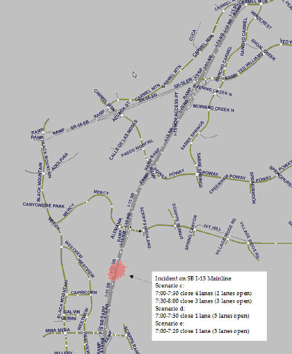
(Source: Cambridge Systematics, Inc.)

Adding active signal control to ramp metering in Scenarios G and H further extends both the emission and system performance benefits. Note that Scenario G outperforms Scenario H in terms of system emissions, even though Scenario H has traveler information added. This is most probably due to the reduced VMT in Scenario G. With traveler information deployed, overall system speeds are improved, but they appear to come at the expense of increased trip length as travelers choose less congested – but more circuitous – routes.

In the incident scenarios (Tables 30 and 31), some routes experience an increase in emissions, due to increased VMT from diversions responding caused by the severe congestion. In fact, VMT is not constant across all scenarios. This is because of the diversion feature in the model. At any time, the route choice model can be reevaluated in order to update the path choices of drivers en route to their destinations. This model also was used to evaluate the response of drivers in incident situations when they are faced with high levels of congestion. When a driver’s path choice is reevaluated, the path costs (e.g., segment travel times) are reconsidered. For driver groups defined in the model parameters as having access to real-time travel information (i.e., informed drivers), an updated travel timetable was used to evaluate path costs. Drivers belonging to a driver group that do not have access to real-time information will reconsider their paths using the same (i.e., historical) travel time information used to evaluate their pretrip paths.

On the I-15 Southbound target section, VMT is substantially higher for Scenario E (incident management plus traveler information) than for either the base or incident management only scenarios. However, the same effect of traveler information is observed here as for the nonincident scenarios, i.e., VMT is higher with traveler information deployed.

The ability of the simulation model to represent the effect traveler information is most likely problematic. Therefore, the Scenario D/Scenario E comparisons cannot be fully trusted. Focusing on just the comparison between Scenario D2 and E2, VHT was reduced by six percent with the addition of incident management on I-15 Southbound. Systemwide CO₂ and other emissions also were reduced as a result of incident management emissions, with CO₂ emissions dropping by over seven percent.

Table 28. Emission results for primary scenarios, 2010 (nonincident scenarios).

6:00 a.m. to 9:00 a.m. – Route	6:00 a.m. to 9:00 a.m. – Scenario	VMT	CO2	Emissions (grams) – CO2 Relative to Base	Emissions (grams) – CO	Emissions (grams) – HC	Emissions (grams) – NOx
Black Mountain Expressway	scenario_A – ramp metering	9,594	7,044,845	4.13%	93,865	2,994	15,448
Black Mountain Expressway	scenario_B – ALINEA ramp metering	9,197	7,008,406	3.59%	96,632	2,915	15,881
Black Mountain Expressway	Base	10,352	6,765,509		95,438	2,806	15,305
Black Mountain Expressway	scenario_G – ramp metering, active signal control	10,812	6,638,842	-1.87%	95,103	2,745	15,306
Black Mountain Expressway	scenario_H – ramp metering, active signal control, traveler information	10,452	6,626,596	-2.05%	94,349	2,776	15,424
Carmel Mountain Expressway	scenario_A – ramp metering	4,309	2,907,180	0.73%	51,873	1,238	6,924
Carmel Mountain Expressway	scenario_B – ALINEA ramp metering	4,361	2,894,335	0.28%	51,591	1,235	6,925
Carmel Mountain Expressway	Base	4,816	2,886,183		51,597	1,228	6,925
Carmel Mountain Expressway	scenario_G – ramp metering, active signal control	4,803	2,723,066	-5.65%	43,797	1,213	5,929
Carmel Mountain Expressway	scenario_H – ramp metering, active signal control, traveler information	4,882	2,937,542	1.78%	52,440	1,250	7,069
I-15 NB	scenario_A – ramp metering	289,513	104,558,162	-4.33%	1,058,182	31,576	239,653
I-15 NB	scenario_B – ALINEA ramp metering	289,598	105,364,626	-3.60%	1,075,848	32,087	240,067
I-15 NB	Base	297,336	109,295,860		1,121,967	33,210	250,478
I-15 NB	scenario_G – ramp metering, active signal control	282,783	104,808,784	-4.11%	1,066,312	31,960	239,578
I-15 NB	scenario_H – ramp metering, active signal control, traveler information	292,487	108,973,584	-0.29%	1,127,518	33,546	247,793
I-15 SB	scenario_A – ramp metering	435,030	213,456,303	-1.73%	1,867,652	80,948	413,619
I-15 SB	scenario_B – ALINEA ramp metering	433,340	208,735,871	-3.91%	1,890,718	76,079	421,936
I-15 SB	Base	420,698	217,218,389		1,954,660	81,830	427,100
I-15 SB	scenario_G – ramp metering, active signal control	421,320	188,302,302	-13.31%	1,823,462	65,871	398,333
I-15 SB	scenario_H – ramp metering, active signal control, traveler information	418,841	203,885,665	-6.14%	1,910,878	74,227	417,795
Other Freeways/Expressways and Major Arterials	scenario_A – ramp metering	81,497	58,168,884	-0.25%	747,604	25,171	122,648
Other Freeways/Expressways and Major Arterials	scenario_B – ALINEA ramp metering	81,160	59,070,832	1.29%	760,056	25,542	125,076
Other Freeways/Expressways and Major Arterials	Base	90,458	58,316,447		753,250	25,153	123,247
Other Freeways/Expressways and Major Arterials	scenario_G – ramp metering, active signal control	93,510	56,799,069	-2.60%	756,325	24,310	121,797
Other Freeways/Expressways and Major Arterials	scenario_H – ramp metering, active signal control, traveler information	94,426	56,399,555	-3.29%	751,274	24,110	121,424
Pomerado Road	scenario_A – ramp metering	28,106	21,551,594	2.00%	244,971	9,468	42,992
Pomerado Road	scenario_B – ALINEA ramp metering	27,850	21,910,938	3.70%	246,868	9,631	43,703
Pomerado Road	Base	31,581	21,129,853		245,072	9,163	43,000
Pomerado Road	scenario_G – ramp metering, active signal control	32,921	17,457,167	-17.38%	231,456	7,224	37,600
Pomerado Road	scenario_H – ramp metering, active signal control, traveler information	35,003	16,982,701	-19.63%	231,020	6,969	37,345
Total, All Highways	scenario_A – ramp metering	848,049	407,686,968	-1.91%	4,064,147	151,395	841,284
Total, All Highways	scenario_B – ALINEA ramp metering	845,506	404,985,008	-2.56%	4,121,713	147,489	853,588
Total, All Highways	Base	855,241	415,612,241		4,221,984	153,390	866,055
Total, All Highways	scenario_G – ramp metering, active signal control	846,149	376,729,230	-9.36%	4,016,455	133,323	818,543
Total, All Highways	scenario_H – ramp metering, active signal control, traveler information	856,091	395,805,643	-4.77%	4,167,478	142,879	846,849

Table 29. System Performance Measures, 6:00 a.m. to 9:00 a.m., 2010 (nonincident scenarios).

Route	Scenario	VMT	VMT Relative to base	VHT	VHT Relative to Base	System Speed
Black Mountain Expressway	scenario_A	9,594	-7.32%	578	13.78%	16.6
Black Mountain Expressway	scenario_B	9,197	-11.16%	547	7.68%	16.8
Black Mountain Expressway	Base	10,352		508		20.4
Black Mountain Expressway	scenario_G	10,812	4.44%	487	-4.13%	22.2
Black Mountain Expressway	scenario_H	10,452	0.97%	513	0.98%	20.4
Carmel Mountain Expressway	scenario_A	4,309	-10.53%	153	1.32%	28.2
Carmel Mountain Expressway	scenario_B	4,361	-9.45%	154	1.99%	28.3
Carmel Mountain Expressway	Base	4,816		151		31.9
Carmel Mountain Expressway	scenario_G	4,803	-0.27%	211	39.74%	22.8
Carmel Mountain Expressway	scenario_H	4,882	1.37%	154	1.99%	31.7
I-15 NB	scenario_A	289,513	-2.63%	4,557	-4.16%	63.5
I-15 NB	scenario_B	289,598	-2.60%	4,652	-2.17%	62.3
I-15 NB	Base	297,336		4,755		62.5
I-15 NB	scenario_G	282,783	-4.89%	4,697	-1.22%	60.2
I-15 NB	scenario_H	292,487	-1.63%	4,910	3.26%	59.6
I-15 SB	scenario_A	435,030	3.41%	18,898	-2.21%	23.0
I-15 SB	scenario_B	433,340	3.01%	16,732	-13.42%	25.9
I-15 SB	Base	420,698		19,325		21.8
I-15 SB	scenario_G	421,320	0.15%	13,260	-31.38%	31.8
I-15 SB	scenario_H	418,841	-0.44%	13,260	-31.38%	31.6
Other Freeways/Expressways and Major Arterials	scenario_A	81,497	-9.91%	3,506	12.82%	23.2
Other Freeways/Expressways and Major Arterials	scenario_B	81,160	-10.28%	3,774	21.43%	21.5
Other Freeways/Expressways and Major Arterials	Base	90,458		3,108		29.1
Other Freeways/Expressways and Major Arterials	scenario_G	93,510	3.37%	3,903	25.60%	24.0
Other Freeways/Expressways and Major Arterials	scenario_H	94,426	4.39%	1,611	-48.15%	58.6
Pomerado Road	scenario_A	28,106	-11.00%	2,479	9.06%	11.3
Pomerado Road	scenario_B	27,850	-11.81%	2,547	12.05%	10.9
Pomerado Road	Base	31,581		2,273		13.9
Pomerado Road	scenario_G	32,921	4.24%	1,409	-38.01%	23.4
Pomerado Road	scenario_H	35,003	10.84%	1,250	-45.01%	28.0
Total, All Highways	scenario_A	848,049	-0.84%	30,171	0.17%	28.1
Total, All Highways	scenario_B	845,506	-1.14%	28,406	-5.69%	29.8
Total, All Highways	Base	855,241		30,120		28.4
Total, All Highways	scenario_G	846,149	-1.06%	23,967	-20.43%	35.3
Total, All Highways	scenario_H	856,091	0.10%	21,698	-27.96%	39.5

Table 30. Emission results for primary scenarios, 2010 (incident scenarios).

6:00 a.m. to 9:00 a.m. – Route	6:00 a.m. to 9:00 a.m. – Scenario	VMT	CO2	Emissions (grams) – CO2 Relative to Base	Emissions (grams) – CO	Emissions (grams) – HC	Emissions (grams) – NOx
Black Mountain Expressway	scenario_D – ramp metering, traveler information	10,510	6,612,747		93,907	2,776	15,239
Black Mountain Expressway	scenario_D2 – ramp metering	10,352	6,630,833		94,364	2,731	15,132
Black Mountain Expressway	scenario_E – ramp metering, incident management, traveler information	11,173	7,012,707	6.05%	99,367	2,966	15,830
Black Mountain Expressway	scenario_E2 – ramp metering, incident management	11,159	7,253,787	9.39%	100,984	3,053	16,385
Carmel Mountain Expressway	scenario_D – ramp metering, traveler information	4,917	2,954,354		52,713	1,256	7,036
Carmel Mountain Expressway	scenario_D2 – ramp metering	4,784	2,859,546		51,033	1,217	6,846
Carmel Mountain Expressway	scenario_E – ramp metering, incident management, traveler information	4,916	2,962,320	0.27%	52,780	1,261	7,094
Carmel Mountain Expressway	scenario_E2 – ramp metering, incident management	4,970	3,054,455	6.82%	54,347	1,304	7,304
I-15 NB	scenario_D – ramp metering, traveler information	293,290	108,978,872		1,120,279	33,379	249,102
I-15 NB	scenario_D2 – ramp metering	297,320	109,779,783		1,129,933	33,453	252,169
I-15 NB	scenario_E – ramp metering, incident management, traveler information	286,463	105,920,289	-2.81%	1,084,187	32,254	242,596
I-15 NB	scenario_E2 – ramp metering, incident management	286,324	106,184,196	-3.28%	1,085,910	32,348	243,117
I-15 SB	scenario_D – ramp metering, traveler information	416,604	208,120,832		1,918,518	76,583	419,330
I-15 SB	scenario_D2 – ramp metering	414,197	211,701,360		1,929,704	80,855	410,968
I-15 SB	scenario_E – ramp metering, incident management, traveler information	430,183	182,615,160	-12.26%	1,831,966	62,389	397,495
I-15 SB	scenario_E2 – ramp metering, incident management	410,096	186,308,356	-11.99%	1,862,559	64,489	403,501
Other Freeways/Expressways and Major Arterials	scenario_D – ramp metering, traveler information	94,486	54,899,300		744,233	23,297	119,262
Other Freeways/Expressways and Major Arterials	scenario_D2 – ramp metering	89,531	57,420,501		744,110	24,812	121,060
Other Freeways/Expressways and Major Arterials	scenario_E – ramp metering, incident management, traveler information	98,903	55,771,900	1.59%	765,045	23,507	122,122
Other Freeways/Expressways and Major Arterials	scenario_E2 – ramp metering, incident management	99,511	58,187,213	1.34%	787,434	24,579	126,858
Pomerado Road	scenario_D – ramp metering, traveler information	34,917	17,214,891		231,881	7,049	37,527
Pomerado Road	scenario_D2 – ramp metering	31,381	21,087,603		243,132	9,221	42,131
Pomerado Road	scenario_E – ramp metering, incident management, traveler information	38,660	18,930,927	9.97%	251,358	7,707	41,510
Pomerado Road	scenario_E2 – ramp metering, incident management	38,750	18,952,848	-10.12%	251,671	7,727	41,691
Total, All Highways	scenario_D – ramp metering, traveler information	854,724	398,780,996		4,161,531	144,340	847,496
Total, All Highways	scenario_D2 – ramp metering	847,565	409,479,626		4,192,276	152,289	848,306
Total, All Highways	scenario_E – ramp metering, incident management, traveler information	870,298	373,213,303	-6.41%	4,084,703	130,084	826,647
Total, All Highways	scenario_E2 – ramp metering, incident management	850,810	379,940,855	-7.21%	4,142,905	133,500	838,856

Table 31. System performance measures, 6:00 a.m. to 9:00 a.m., 2010 (incident scenarios)

Route	Scenario	VMT	VMT Relative to Base	VHT	VHT Relative to Base	System Speed (mph)
Black Mountain Expressway	scenario_D	10,510		474		22.2
Black Mountain Expressway	scenario_D2	10,352		462		22.4
Black Mountain Expressway	scenario_E	11,173	6.31%	481	1.48%	23.2
Black Mountain Expressway	scenario_E2	11,159	7.80%	464	0.43%	24.0
Carmel Mountain Expressway	scenario_D	4,917		156		31.5
Carmel Mountain Expressway	scenario_D2	4,784		215		22.3
Carmel Mountain Expressway	scenario_E	4,916		160		30.7
Carmel Mountain Expressway	scenario_E2	4,970		158		31.5
I-15 NB	scenario_D	293,290		4,789		61.2
I-15 NB	scenario_D2	297,320		5,113		58.1
I-15 NB	scenario_E	286,463	-2.33%	4,877	1.84%	58.7
I-15 NB	scenario_E2	286,324	-3.70%	5,024	-1.74%	57.0
I-15 SB	scenario_D	416,604		17,879		23.3
I-15 SB	scenario_D2	414,197		25,322		16.4
I-15 SB	scenario_E	430,183	3.26%	16,637	-6.95%	25.9
I-15 SB	scenario_E2	410,096	-0.99%	23,781	-6.09%	17.2
Other Freeways/Expressways and Major Arterials	scenario_D	94,486		3,155		30.0
Other Freeways/Expressways and Major Arterials	scenario_D2	89,531		3,799		23.6
Other Freeways/Expressways and Major Arterials	scenario_E	98,903	4.67%	3,284	4.10%	30.1
Other Freeways/Expressways and Major Arterials	scenario_E2	99,511	11.15%	3,994	5.13%	24.9
Pomerado Road	scenario_D	34,917		1,161		30.1
Pomerado Road	scenario_D2	31,381		1,324		23.7
Pomerado Road	scenario_E	38,660	10.72%	1,201	3.45%	32.2
Pomerado Road	scenario_E2	38,750	23.48%	1,404	6.04%	27.6
Total, All Highways	scenario_D	854,724		27,614		31.0
Total, All Highways	scenario_D2	847,565		36,235		23.4
Total, All Highways	scenario_E	870,298	1.82%	26,640	-3.53%	32.7
Total, All Highways	scenario_E2	850,810	0.38%	34,825	-3.89%	24.4

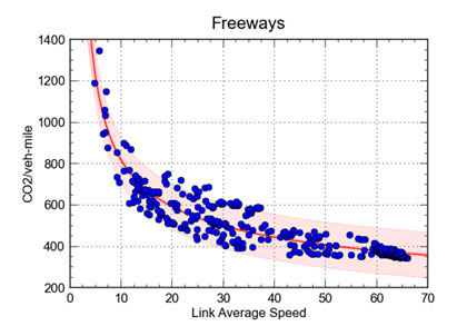
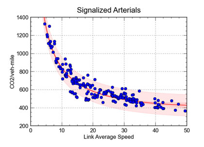
Figures 36 and 37 were developed from the link-level MOVES output for all scenarios to see if the results were reasonable. The freeway curve in Figure 36 mimics that shown in Barth and Boriboonsomsin, which was developed with independent data. (Barth, Matthew and Boriboonsomsin, Kanok, “Real World CO₂ Impacts of Traffic Congestion,” submitted to Transportation Research Board Annual Meeting, 2008.) For a given speed value (for speeds above about 15 mph), there is a spread in the data indicating that different operating modes are being used. Note that the freeway curve stops at 65 mph – the data in Barth and Boriboonsomsin show that the curve turns positive at speeds above 70 mph.

Figure 36. Scatter graph. CO₂ emission rates from MOVES outputs, freeways.

(Source: Cambridge Systematics, Inc.)

Figure 37. Scatter graph. CO₂ emission rates from MOVES outputs, arterials.

(Source: Cambridge Systematics, Inc.)

Variable Speed Limit Scenarios

Because VSL is relatively new and some of its potential benefits have been called into question, it was first decided to test the traffic flow effects of VSL before proceeding to emissions analysis. As shown below, we could not find any appreciable traffic flow effect in this corridor for VSL treatment, Therefore, we did not conduct any emissions analysis.

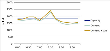
Two profiles are used in the analysis of the VSL strategies, they are shown below compared to the capacity at the bottleneck (Figure 38).

Figure 38. Line graph. Demand profile at the analysis bottleneck.

(Source: Cambridge Systematics, Inc.)

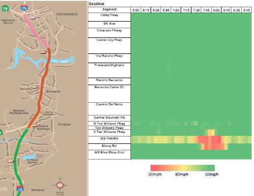
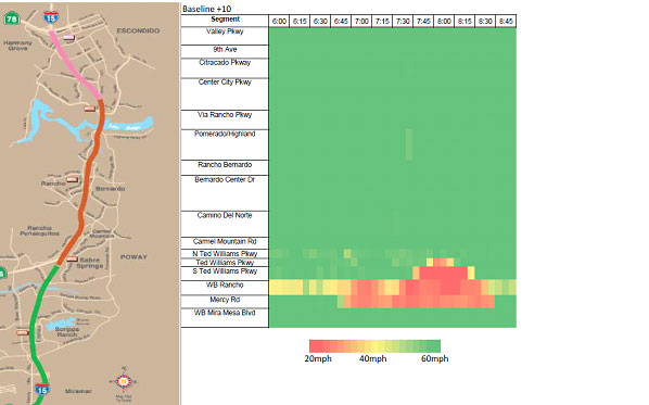
The congestion along the corridor under the two demand profiles is represented by the speed plots below (Figures 39 and 40).

Figure 39. Map and graph. Speed profile under normal demand, no VSL.

(Source: Cambridge Systematics, Inc.)

Figure 40. Map and graph. Speed profile under high demand, no VSL.

(Source: Cambridge Systematics, Inc.)

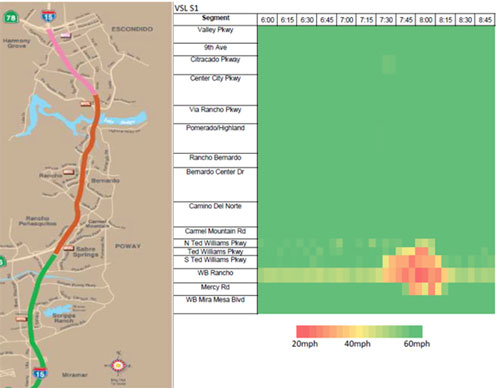
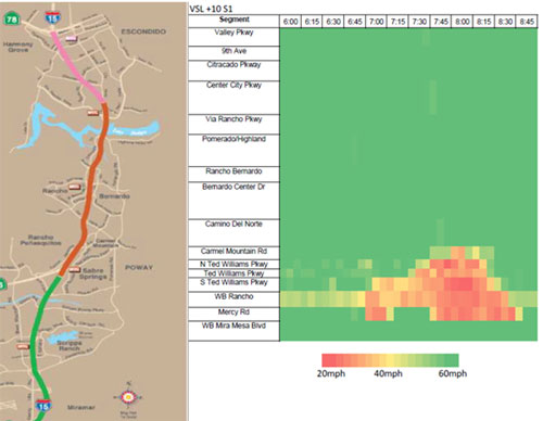
The first VSL strategy applied to the corridor is a standard VSL strategy aimed at improving safety at the upstream end of the queue where heavy and unanticipated breaking occur. VSL signs are positioned upstream of the bottleneck every 1,000 feet. When speeds drop below 45 mph a message warning of congestion is displayed. And, when a speed drop below 30 mph is detected downstream the VSL sign changes to 30 mph and the upstream VSL sign changes to 45 mph. This strategy therefore follows the back of the queue first warning with a 45 mph speed restriction and then a 30 mph speed restriction.

The congestion when applying this strategy is shown below using speed plots (Figures 41 and 42).

Figure 41. Map and graph. Speed profile under normal demand with traditional VSL.

(Source: Cambridge Systematics, Inc.)

Figure 42. Map and graph. Speed profile under high demand with traditional VSL.

(Source: Cambridge Systematics, Inc.)

The traditional VSL strategy elongated the congestion physically and temporally, while reducing the intensity of the speed decreases within the congested area. The next measure analyzed is delay. A comparison of delay along the corridor (Table 32) will indicate whether the freeway performance is improved by the VSL strategy.

Table 32. Freeway delay (vehicle hours).

	Normal Demand	High Demand
No VSL	540	990
Traditional VSL	600	1,120

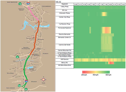
The second VSL strategy is a nontraditional strategy, one that attempts to reduce congestion at a bottleneck by “metering” mainline volume miles upstream of the bottleneck. For this study the nontraditional strategy was applied approximately 4.5 miles upstream of the bottleneck, 1 mile upstream of the maximum extent of the queue under normal conditions.

The nontraditional VSL strategy was applied over approximately 5.5 miles of mainline freeway and was responsive to traffic conditions at the bottleneck location. When speeds at the bottleneck dropped below 30 mph the VSL strategy was applied, when they increased to between 30 mph and 45 mph the VSL signs changed from 30 mph to 45 mph and when the speeds increased above 45 mph the VSL strategy stopped. Warning upstream of the upcoming VSL signs was given throughout the application of the strategy.

The speed profiles for the application of the nontraditional VSL strategy are shown for both the normal and high-demand scenario (Figures 43 and 44).

Figure 43. Map and graph. Speed profile under normal demand with nontraditional VSL.

(Source: Cambridge Systematics, Inc.)

Figure 44. Map and graph. Speed profile under high demand with nontraditional VSL.

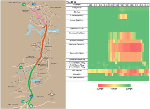
(Source: Cambridge Systematics, Inc.)

In both the normal and high-demand scenarios the nontraditional VSL strategy successfully reduced the size duration of congestion at the bottleneck location. But, as the delay results show (Table 33), the total freeway delay is greater than both the existing condition and traditional VSL strategy. This is likely due to the great extent over which the nontraditional VSL strategy was applied as well as the unforeseen bottleneck that appears at Bernardo Center Dr. when the strategy is applied in the high-demand scenario.

Table 33. Freeway delay (vehicle hours).

	Normal Demand	High Demand
No VSL	540	990
Traditional VSL	600	1,120
Nontraditional VSL	690	2,000

These results indicate that VSL, as applied in this corridor, has no appreciable effect on overall delay.

Modeling Challenges and Limitations

Vehicular emissions are a result of two interacting factors: amount of travel (VHT) and the driving profiles of the vehicles involved. Microsimulation models do an excellent job at capturing system performance measures because they model individual vehicle movements. They also can provide modal activity of vehicles, but they have not been calibrated to provide second-by-second vehicle trajectories but rather have been calibrated to system performance. This is a limitation of the models used in this analysis. Therefore, the degree that simulation models replicate vehicle trajectories is not known – this a limitation of the analysis.

VMT fluctuates from run-to-run, even when there is only a slight difference between runs (e.g., the two types of ramp metering in Scenarios A and B). As previously discussed, the TransModeler application used in this study assigns a trip table (demand between origins and destinations) using the stochastic user equilibrium approach, so some differences in VMT will result from the assignment process. This is to be expected, as it more realistically represents how travelers behave, but it makes isolation of the improvements’ effects difficult. Transmodeler also has a feature that allows simulation of traveler information. In our tests, we observed erratic behavior in this algorithm for the incident scenarios, in terms of widely different network VMT. We are uncertain how realistically this algorithm behaves, and identify the incident scenarios with traveler information as an improvement as problematic.

You may need the Adobe® Reader® to view the PDFs on this page.