Travel and Emissions Impacts of Highway Operations Strategies
Chapter 6. Long-Term Regional Impacts of Operations Strategies
Introduction
The I-15 simulation analysis established the short-term emissions benefits of operations strategies. However, the main impetus for conducting the study was to determine if improvements due to operations strategies changed long-term traveler behavior, and the degree to which behavioral changes impact the effectiveness of operations strategies. Specifically, is VMT over the long term increased due to less congested travel caused by operational improvements.
As discussed in Chapter 1, a decision to direct the project toward an advanced modeling framework to study long-term travel behavior changes was made. Initially it was thought that the SHRP 2 C10B, Partnership to Develop an Integrated, Advanced Travel Demand Model and a Fine-grained, Time-Sensitive Network, would be used. SHRP 2 C10B was underway at the same time as this project, but its original schedule showed that its scenario testing would coincide with this project. Unfortunately, SHRP 2 C10B experienced a long scheduling delay which put it out reach of this project. Also, because it was an experimental framework, it also experienced convergence problems during its operation.
For these reasons, an alternative modeling framework was chosen. The travel demand model framework developed by the Metropolitan Transportation Commission (MTC), the MPO for the San Francisco Bay Area for several reasons:
- It is an activity-based model, which reflects trip-making in a realistic way.
- The UrbanSim land use model, one of the most sophisticated models of its kind, provides land use “simulation” where one of the inputs is the performance of the transportation system.
- Team member Urban Analytics could easily adapt its original reliability research (Chapter 4) to the UrbanSim model, providing a way to incorporate reliability into long-term travel decisions.
The MTC model’s main shortcoming is that it uses traditional traffic assignment methods to estimate system performance. However, the primary output desired from the model is the change in demand. Also, postprocessors were developed to refine the speed estimates, calculate emissions, and produce reliability statistics (see below).
Methodology
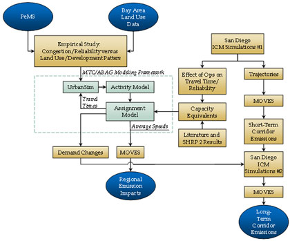
The methodology for this approach is summarized in Figure 45. In this chapter, we provide the details on the method.
Figure 45. Flowchart. Final study approach, advanced modeling phase.
(Source: Cambridge Systematics, Inc.)
Operations Strategies Considered
The following five deployment scenarios were studied with the MTC model:
- Scenario 1: Active Signal Control (major arterials).
- Scenario 2: Ramp Meters (freeways).
- Scenario 3: Incident Management (freeways).
- Scenario 4: Active Traffic and Demand Management (ATDM; freeways).
- Scenario 5: ATDM + Signal Control.
The reliability research presented in Chapter 4 indicated that the East Bay area had many highways that would be considered to be unreliable. Therefore, the deployment of these strategies was confined to Alameda and Contra Costa counties but included all the applicable highways in those counties.
Analytical Basis for Studying Operations Strategies
Economic theory holds that, among many other factors, long-term changes in travel behavior – in terms of additional and/or longer trips – are a function of developers and travelers responding to system conditions. If conditions are improved, travel increases because developers and travelers change their behavior to take advantage of lower travel costs. Likewise, if conditions degrade, travel is suppressed, according to theory. Traditionally, the measure of network performance used to estimate shifts in travel behavior is average (or typical) travel time. Recently however, it has been noted that travel-time reliability – how travel time varies due to variability in the underlying causal factors of congestion – also is an important consideration that affects developers’ and travelers’ behavior. The research presented in Chapter 4 documents the changes on land use patterns caused by this effect.
Reliability is affected not only by the disruptions caused by events like incidents, inclement weather, and work zones but also by demand and its interaction with physical capacity. In fact, reliability is a function of the interaction of all these factors. (Kittelson Associates et al., “SHRP 2 – L08: Incorporation of Travel-time reliability into the HCM. Final Report,” Transportation Research Board, April 2013.) (Cambridge Systematics et al., SHRP 2 – L03: Analytic Procedures for Determining the Impacts of Reliability Mitigation Strategies, Transportation Research Board, 2013.) The implication of this is that any strategy that affects disruptions, demand, or capacity will have an effect on reliability, albeit to different degrees. Further, research has shown that the average travel time is correlated with common measures of reliability (e.g., 95th percentile travel time).
The mechanisms for affecting travel time within travel demand models – or macroscopic and mesoscopic simulations models for that matter – is to change link capacity or volume. For capital expansion projects (e.g., more through lanes, interchange reconstruction) capacity is directly affected. In travel demand models, the change in capacity results in a change in travel time that then affects traveler behavior. A large number of past studies have documented the decrease in travel times and delay due to implementing operations strategies. A few studies also have shown that operations strategies also improve reliability, in addition to reducing overall delay. Therefore, to model the reduction in travel times caused by operations strategies (at least the ones studied here), we have chosen to translate their effects through capacity increases. Our rationale for taking this approach is given below.
It would have been desirable to have both travel time and reliability in a model affecting travel behavior, and methods to estimate this change exist and were applied for the land use portion of the framework. However, the ABM portion is not currently capable of using this information. In Chapter 2 we reviewed some of the recent work on the valuation of reliability and its inclusion in models, primarily undertaken in the SHRP 2 program. The concept put forth is that reliability should be considered as an extra factor in the utility function used to derive travel demand – essentially this increases the total cost associated with a travel choice. Chapter 2 also proposed a simple way to accommodate this factor by constructing a travel time equivalent, the sum of the average/typical travel time and a reliability component that is scaled using a reliability ratio (value of reliability to travelers divided by the value of average time).
However, when we approached the two MPOs involved in this study (Sacramento Council of Governments, which was involved in SHRP 2 C10B, and MTC), they were highly reluctant to use travel time equivalents as part of the feedback loop because their models had been calibrated to average travel times only. Until travel demand models, especially activity-based ones, include reliability implicitly when they are initially developed, adding reliability to travel decisions at their source will have to wait. As discussed in the next subchapter, an approximation for this effect has been included and tested in several MPO models, including MTC’s. This approximation basically shifts the volume-delay function used in traffic assignment to the left, which has the same effect as the travel time equivalent approach: it increases travel time, i.e., the cost associated with travel.
The mechanism we have chosen to study the effects of operations strategies is capacity. In some cases, operations strategies directly affect capacity (e.g., ramp metering, junction control, hard shoulder running). Incident management and work zone management also affect capacity directly, although the effect is in terms of reduction of the time that capacity was lost. Studies of active signal control systems most often define the effect in terms of increased speeds or reduced delay, although the mechanism by which this achieved is more efficiently signal timing, which has the practical effect of increasing throughput (capacity) at signals. So, it is not a stretch to use capacity as the means for modeling the effects of the operations strategies studied here.
Even though the travel behavior effects of reliability are handled only crudely, the current study did conduct original research on the effect of reliability on land use, and subsequently incorporated it into the MTC modeling framework.
Determining Capacity Equivalents for Operations Strategies
Because the MTC travel model uses a traditional traffic assignment process, the ability to model traffic flow is limited. The model is only sensitive to free-flow speed and volume-to-capacity (v/c) ratios, and since volume is derived by the model, capacity is the only practical way to replicate the effect of operations within the model.
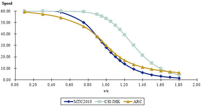
Traffic assignment procedures use speed-flow functions (sometimes called volume-delay functions) to compute the impedance on links in the network. The higher the impedance, they less likely vehicles are to be assigned to a particular link. While v/c is the only independent variable in a speed-flow function (assuming that free-flow speed is fixed), a variety of functional forms have been used to fit speed-flow functions. Most of the earlier forms were built around modeling recurring (i.e., those related strictly to volumes and physical capacity) conditions. An example is the original Bureau of Public Roads (BPR) function and several variations on it, such as the one developed by Cambridge Systematics and JHK Associates in the early 1990s (Figure 46):
Figure 46. Equation. Speed.

(Source: Speed Adjustments Using Volume-Delay Functions, TMIP Technical Synthesis, January 2009.)
These earlier forms eventually came under criticism for not replicating measured conditions in the field. This led, for example, to work by the Atlanta Regional Commission (ARC) to develop a conical form of the function that matched data from ITS detectors fairly well. It should be pointed out that the field data included the effect of nonrecurring congestion sources, because it was continuously collected, so the net effect is to have a way to estimate overall average speeds from just the v/c ratio. MTC currently uses a variant of the BPR function for freeways that is almost identical in its prediction to the ARC conical model:
Figure 47. Equation. Speed.

(Source: MTC Technical Memo, March 6, 2012.)
The MTC reformulation also is based on matching predicted speeds to ITS detector data. Both the ARC and MTC functions predict much lower speeds than traditional functions at the same v/c value. This has the effect of at least loosely accounting for the effect of nonrecurring congestion in the assignment process. It also leads to gradually increasing impedance for v/cs less than 1.0 which may help with convergence.
A more direct account of nonrecurring factors was recently completed by the Puget Sound Regional Council (PSRC). (Puget Sound Regional Council, Benefit-Cost Analysis: General Methods and Approach, July 2009, Updated March 2010.) They developed an “certainty-equivalent delay penalty” that is added to their usual volume delay function; this has the effect if shifting the function slightly to the left.
The ARC, MTC, andPSRC activities all account for nonrecurring sources in general, but do not provide a way to estimate the impacts that operations strategies have. For that, the effects of operations must be translated in terms of capacity. In fact, MTC currently does this for ramp metering on freeways and signal coordination on arterials:
- Ramp metering capacity:
- 2,150 passenger cars per hour per lane (pcphpl) (compared to 2,050 for CBD).
- 2,200 pcphpl (compared to 2,100 for urban and 2,150 for suburban).
- Signal Coordination:
- 1,050 pcphpl (compared to 1,000).
Translating operations effects into capacity equivalents can sometimes be direct (e.g., ramp metering) if field studies have been done. In other cases, it is necessary to derive the capacity equivalent analytically. Studies usually report delay, and sometimes reliability, savings due to operational improvements. The challenge then becomes “what equivalent physical capacity increase would have produced the delay savings”? A simple approach to doing this uses a BPR variant that is focused on recurring delay; in this case we have chosen the CS/JHK function because it mimics the steepness of many functions currently in use when v/c > 1.0. For this analysis, we assume that the delay savings accrue in congested conditions at v/c = 1.1. We first estimate the delay at v/c = 1.1, reduce the delay by percentage reduction from a previous study, find the new v/c level that corresponds to that delay, and calculate the capacity increase that would produce the new v/c value.
Figure 48. Graph. Comparison of selected speed-flow curves.
(Source: Cambridge Systematics, Inc.)
For incidents, the situation is more complex because the delay savings do not accrue to the recurring portion of delay. For this we need to estimate both recurring and incident delay. The ITS Deployment Analysis System (IDAS) has a series of tables that estimate incident delay as a function of v/c and number of lanes. These were developed with a stochastic procedure using data from incident management systems on incident duration and lane blockages. Equations were fit to these data for this project:
Figure 49. Equation. Two-lane freeways.

(Source: Cambridge Systematics, IDAS User’s Manual, 2009.)
Figure 50. Equation. Three-lane freeways.

(Source: Cambridge Systematics, IDAS User’s Manual, 2009.)
Figure 51. Equation. Four-lane freeways.

(Source: Cambridge Systematics, IDAS User’s Manual, 2009.)
Where:
Du = incident delay rate, hours per mile
X = v/c; max = 1.0
Using both the BPR (the CS/JHK equation) and IDAS curves provides an estimate of total delay. At v/c = 1.1, the total delay rate is 0.0409 hours per mile (0.0199 for incident delay plus 0.0210 for recurring delay). The corresponding value that the BPR curve would predict this delay rate for is v/c = 1.365. The effect of incident management strategies is most often to reduce incident duration. This can be accounted for by taking advantage of the fact that incident delay is a function of the square of incident duration (H. Cohen and F. Southworth (1999) On the measurement and valuation of travel time variability due to incidents on freeways. Journal of Transportation and Statistics 2.2: 123-132. Also, the University of Maryland, as part of the ongoing CHART evaluations, developed a predictive equation model based on running experiments with microscopic simulation where the exponent on incident duration is 1.78.):
Figure 52. Equation. Adjusted incident delay.

(Source: Cambridge Systematics, IDAS User’s Manual, 2009.)
Where:
Rd = Percent reduction in incident duration
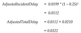
With this knowledge, a new incident delay and total delay is computed, the v/c value predicted by the BPR function is found, and percent increase in capacity that would produce this value is calculated. Continuing the example, assuming a 25 percent decrease in incident duration is effected by incident management and two lanes in one direction:
Figure 53. Equation. Adjusted incident delay; adjusted total delay.
(Source: Cambridge Systematics, Inc.)
The v/c value that would produce a delay rate of 0.0322 using the BPR function is 1.280. Therefore, there is a 7 percent capacity increase due to an incident management program that reduces incident duration by 25 percent.
A summary of the capacity equivalents for the operations strategies to be studied is shown in Table 34.
Table 34. Capacity equivalents for operations strategies.
| Operations Strategy |
Capacity Equivalent and Justification |
| Ramp metering |
Three percent; Zhang, L. and D. Levinson. Ramp Metering and Freeway Bottleneck Capacity. Transportation Research: A Policy and Practice 44(4), May 2010, pp. 218-235. |
| Incident Management |
Two unidirectional lanes: 7 percent Three plus unidirectional lanes: 6 percent; based on empirical delay analysis and 25 percent reduction in incident duration |
| Active signal control |
Seven percent; based on empirical delay analysis assuming that active signal control reduced delay by 25 percent (MTC value is 5 percent capacity increase) |
| ATDM |
Twenty percent; meant cover multiple improvement types, including ramp metering, lane control, queue warning, junction control, and traveler information (Synthesis of Active Traffic Management Experiences in Europe and the United States) |
Modeling Steps
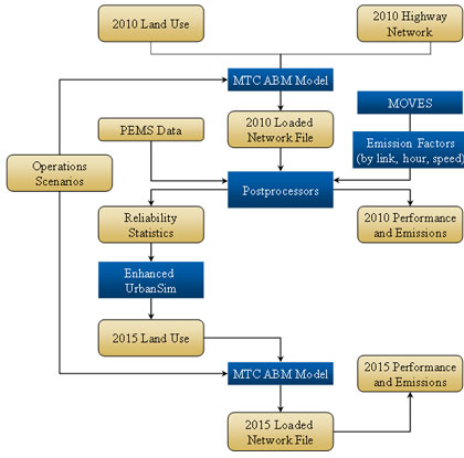
The modeling sequence starts with the 2010 base conditions for land use and network state from the most recent application of the model by MTC (Figure 54). It was determined that only one iteration of the entire framework (2015) should be attempted because it was uncertain how the reliability-modified version of UrbanSim would behave. Therefore, to replicate the effect of increased congestion in future years, it was decided to adjust the volume-delay functions for freeways and major arterials to induce extra congestion; this was done my adding a factor that increased the v/c ratio by 30 percent.
Figure 54. Flowchart. Regional emission modeling using the MTC model.
(Source: Cambridge Systematics, Inc.)
The output of the model produced a loaded network file that was postprocessed. First, because the MTC model works on periods of the day, the assigned volume was broken out to individual hours using factors developed by MTC. Then, hourly speeds were estimated with MTC’s volume-delay functions. The MOVES model was run to develop hourly emission rates by speed range for the AM peak period (the period chosen for study), and emissions were calculated by link.
A separate postprocessor was used to develop reliability statistics for feedback into the UrbanSim model. For this, we used the finding that reliability statistics can be related to the mean travel time. Using PeMS data, functions to predict the median and 80th percentile travel times from the mean travel were developed individually for I-580 and I-880 in Alameda and Contra Costs counties. Other freeways used the I-880 function and signalized arterials used the relationship developed by SHRP 2 Project L03. The median and 80th percentile travel times are used in the enhanced version of UrbanSim as the measure of the reliability “space.”
The modeling using the enhanced UrbanSim/MTC model provides an estimate of the regional impact of operations strategies on emissions and performance. However, because performance is based on volume-delay functions rather than more sophisticated traffic modeling, performance and emissions estimates are crude. Because travel demand models are geared to estimating demand rather than performance, we use the changes in VMT that result from deploying operations strategies to modify the demand used in the I-15 simulation tests.
Regional Modeling Results
Base Year (2010) Results, AM Peak Period
Table 35 shows the results of the 2010 model runs for the base case and each scenario for the AM peak period (6:00 to 10:00 a.m.). Regionally, under most scenarios, emissions generally decrease by a fractional amount (less than one percent). CO2 emissions decrease fractionally for all scenarios except for ramp meters. VMT increases proportionately to the “aggressiveness” of the operations strategy. Likewise, VHT decreases proportionately to the aggressiveness strategy. The net effect is that although the deployment of operations leads to increased VMT, the increase is small enough – and the benefit of operations is large enough – that emissions drop marginally in the short run.
The VMT increase is likely due to changes in demand patterns predicted by the activity-based portion of the model. The MTC model is set up to perform four iterations for each model run. At the end of each iteration, the traffic assignment results are fed back to the ABM and travel behavior is updated. The improved travel conditions created by the operations strategies are leading to changes in demand patterns. The largest increases occur within the treatment area (Alameda and Contra Costa counties) but VMT also increases in adjacent counties.
What are the sources of the VMT increase? As shown back in Table 4, several possible sources exist. In addition to rerouting during the traffic assignment phase – which is actually likely to be close to zero – VMT in the ABM also can be affected by:
- Time of Day/Schedule (peak spreading).
- Destination/Stop Location (improved accessibility effect combined with negative pricing effect on trip distribution for nonwork trips.
- Joint Travel Arrangements (planned carpool/escorting).
- Tour Frequency, Sequence, and Formation of Trip Chains (lower tour frequency and higher chaining propensity).
- Daily Pattern Type (more compressed workdays and work from home).
- Usual Locations and Schedule for Nonmandatory Activities (compressed/chain patterns).
Table 35. AM peak period performance results, 2010 MTC Model runs.
 |
VHT |
VMT |
HC (grams) |
CO (grams) |
NOx (grams) |
CO2 (grams) |
County |
Highway Type |
| Base |
343,568 |
11,582,560 |
1,262,663 |
27,083,364 |
11,169,580 |
6,210,504,349 |
Remainder of Area |
Freeway |
| Base |
152,840 |
2,166,450 |
392,671 |
6,271,028 |
2,855,753 |
1,606,732,330 |
Remainder of Area |
Expressway |
| Base |
63,818 |
1,589,041 |
185,509 |
3,645,045 |
1,146,570 |
809,213,677 |
Remainder of Area |
Collector |
| Base |
187,652 |
5,210,839 |
551,201 |
11,294,481 |
3,423,125 |
2,481,248,722 |
Remainder of Area |
Arterial |
| Base |
305,635 |
8,348,239 |
1,015,974 |
20,080,531 |
8,045,557 |
4,687,953,422 |
Alameda/Contra Costa |
Freeway |
| Base |
73,648 |
329,299 |
84,589 |
1,105,842 |
618,699 |
309,503,463 |
Alameda/Contra Costa |
Expressway |
| Base |
53,062 |
1,058,754 |
141,071 |
2,595,094 |
820,211 |
587,490,181 |
Alameda/Contra Costa |
Collector |
| Base |
130,908 |
3,350,238 |
367,297 |
7,420,142 |
2,183,500 |
1,638,131,995 |
Alameda/Contra Costa |
Arterial |
| Base |
1,311,129 |
33,635,421 |
4,000,976 |
79,495,527 |
30,262,996 |
18,330,778,140 |
|
|
| S1: Active Signal Control |
343,304 |
11,576,688 |
1,261,320 |
27,070,528 |
11,161,438 |
6,204,976,096 |
Remainder of Area |
Freeway |
| S1: Active Signal Control |
152,513 |
2,168,006 |
393,927 |
6,284,369 |
2,861,256 |
1,611,175,680 |
Remainder of Area |
Expressway |
| S1: Active Signal Control |
63,757 |
1,587,687 |
185,412 |
3,642,553 |
1,145,518 |
808,732,230 |
Remainder of Area |
Collector |
| S1: Active Signal Control |
187,782 |
5,213,571 |
552,483 |
11,308,731 |
3,428,449 |
2,485,652,547 |
Remainder of Area |
Arterial |
| S1: Active Signal Control |
305,111 |
8,345,165 |
1,016,681 |
20,088,493 |
8,049,673 |
4,690,034,745 |
Alameda/Contra Costa |
Freeway |
| S1: Active Signal Control |
72,670 |
332,532 |
85,370 |
1,116,542 |
623,106 |
312,544,663 |
Alameda/Contra Costa |
Expressway |
| S1: Active Signal Control |
52,877 |
1,053,423 |
140,256 |
2,580,578 |
816,039 |
584,211,094 |
Alameda/Contra Costa |
Collector |
| S1: Active Signal Control |
124,947 |
3,370,896 |
357,639 |
7,319,342 |
2,164,664 |
1,609,086,110 |
Alameda/Contra Costa |
Arterial |
| S1: Active Signal Control |
1,302,960 |
33,647,967 |
3,993,088 |
79,411,136 |
30,250,142 |
18,306,413,165 |
|
|
| S1: Active Signal Control |
-0.623% |
0.037% |
-0.197% |
-0.106% |
-0.042% |
-0.133% |
Compared to Base |
|
| S2: Ramp Meters |
346,028 |
11,588,102 |
1,267,989 |
27,138,783 |
11,191,204 |
6,225,734,233 |
Remainder of Area |
Freeway |
| S2: Ramp Meters |
153,101 |
2,167,932 |
394,120 |
6,287,219 |
2,861,918 |
1,611,906,308 |
Remainder of Area |
Expressway |
| S2: Ramp Meters |
63,827 |
1,588,017 |
185,416 |
3,643,397 |
1,145,680 |
808,765,334 |
Remainder of Area |
Collector |
| S2: Ramp Meters |
188,345 |
5,220,900 |
553,344 |
11,327,560 |
3,433,396 |
2,489,216,990 |
Remainder of Area |
Arterial |
| S2: Ramp Meters |
297,062 |
8,460,037 |
1,002,540 |
20,169,985 |
8,059,392 |
4,676,599,450 |
Alameda/Contra Costa |
Freeway |
| S2: Ramp Meters |
72,998 |
328,837 |
84,117 |
1,099,443 |
616,529 |
307,991,828 |
Alameda/Contra Costa |
Expressway |
| S2: Ramp Meters |
52,743 |
1,052,670 |
140,396 |
2,581,347 |
815,703 |
584,517,697 |
Alameda/Contra Costa |
Collector |
| S2: Ramp Meters |
130,342 |
3,339,830 |
365,492 |
7,387,607 |
2,174,084 |
1,631,048,141 |
Alameda/Contra Costa |
Arterial |
| S2: Ramp Meters |
1,304,446 |
33,746,325 |
3,993,413 |
79,635,341 |
30,297,906 |
18,335,779,980 |
|
|
| S2: Ramp Meters |
-0.510% |
0.330% |
-0.189% |
0.176% |
0.115% |
0.027% |
Compared to Base |
|
| S3: Incident Management |
348,499 |
11,593,971 |
1,267,048 |
27,139,371 |
11,188,287 |
6,225,503,367 |
Remainder of Area |
Freeway |
| S3: Incident Management |
151,787 |
2,167,842 |
393,847 |
6,285,265 |
2,859,813 |
1,611,041,911 |
Remainder of Area |
Expressway |
| S3: Incident Management |
63,698 |
1,587,486 |
185,388 |
3,642,163 |
1,145,529 |
808,634,827 |
Remainder of Area |
Collector |
| S3: Incident Management |
188,183 |
5,221,420 |
552,147 |
11,316,489 |
3,429,792 |
2,485,388,776 |
Remainder of Area |
Arterial |
| S3: Incident Management |
283,147 |
8,699,197 |
983,904 |
20,462,131 |
8,132,149 |
4,690,061,565 |
Alameda/Contra Costa |
Freeway |
| S3: Incident Management |
65,373 |
326,527 |
82,844 |
1,087,757 |
608,524 |
304,213,797 |
Alameda/Contra Costa |
Expressway |
| S3: Incident Management |
51,450 |
1,023,921 |
136,540 |
2,509,287 |
792,482 |
568,280,085 |
Alameda/Contra Costa |
Collector |
| S3: Incident Management |
124,894 |
3,261,390 |
352,626 |
7,161,690 |
2,111,122 |
1,579,060,291 |
Alameda/Contra Costa |
Arterial |
| S3: Incident Management |
1,277,032 |
33,881,754 |
3,954,345 |
79,604,153 |
30,267,697 |
18,272,184,619 |
|
|
| S3: Incident Management |
-2.601% |
0.732% |
-1.165% |
0.137% |
0.016% |
-0.320% |
Compared to Base |
|
| S4: ATDM |
352,870 |
11,609,056 |
1,272,211 |
27,205,182 |
11,211,086 |
6,242,479,060 |
Remainder of Area |
Freeway |
| S4: ATDM |
153,064 |
2,171,283 |
395,736 |
6,307,951 |
2,867,549 |
1,617,681,290 |
Remainder of Area |
Expressway |
| S4: ATDM |
63,867 |
1,589,828 |
185,694 |
3,647,890 |
1,147,416 |
809,939,561 |
Remainder of Area |
Collector |
| S4: ATDM |
188,799 |
5,228,478 |
554,219 |
11,345,428 |
3,438,179 |
2,493,008,923 |
Remainder of Area |
Arterial |
| S4: ATDM |
273,187 |
8,951,921 |
977,672 |
20,909,871 |
8,248,298 |
4,737,912,890 |
Alameda/Contra Costa |
Freeway |
| S4: ATDM |
58,518 |
322,420 |
75,954 |
1,033,198 |
566,116 |
283,574,694 |
Alameda/Contra Costa |
Expressway |
| S4: ATDM |
50,456 |
1,001,101 |
133,653 |
2,454,651 |
774,466 |
555,894,433 |
Alameda/Contra Costa |
Collector |
| S4: ATDM |
121,446 |
3,199,702 |
344,583 |
7,006,472 |
2,068,064 |
1,545,170,047 |
Alameda/Contra Costa |
Arterial |
| S4: ATDM |
1,262,207 |
34,073,788 |
3,939,722 |
79,910,643 |
30,321,173 |
18,285,660,898 |
|
|
| S4: ATDM |
-3.731% |
1.303% |
-1.531% |
0.522% |
0.192% |
-0.246% |
Compared to Base |
|
| S5: ATDM + Signal Control |
352,669 |
11,610,621 |
1,274,067 |
27,220,404 |
11,218,758 |
6,247,910,589 |
Remainder of Area |
Freeway |
| S5: ATDM + Signal Control |
152,536 |
2,169,793 |
394,662 |
6,295,738 |
2,863,252 |
1,613,924,954 |
Remainder of Area |
Expressway |
| S5: ATDM + Signal Control |
63,795 |
1,589,268 |
185,601 |
3,646,582 |
1,146,597 |
809,546,694 |
Remainder of Area |
Collector |
| S5: ATDM + Signal Control |
188,374 |
5,226,018 |
553,884 |
11,339,755 |
3,436,200 |
2,491,593,743 |
Remainder of Area |
Arterial |
| S5: ATDM + Signal Control |
270,505 |
8,927,788 |
968,088 |
20,810,332 |
8,197,204 |
4,708,591,041 |
Alameda/Contra Costa |
Freeway |
| S5: ATDM + Signal Control |
57,024 |
323,500 |
76,256 |
1,038,153 |
567,250 |
284,740,324 |
Alameda/Contra Costa |
Expressway |
| S5: ATDM + Signal Control |
49,828 |
993,879 |
132,750 |
2,437,782 |
769,081 |
552,052,770 |
Alameda/Contra Costa |
Collector |
| S5: ATDM + Signal Control |
115,612 |
3,208,040 |
334,226 |
6,886,853 |
2,043,228 |
1,512,451,075 |
Alameda/Contra Costa |
Arterial |
| S5: ATDM + Signal Control |
1,250,344 |
34,048,907 |
3,919,535 |
79,675,599 |
30,241,569 |
18,220,811,190 |
|
|
| S5: ATDM + Signal Control |
-4.636% |
1.229% |
-2.036% |
0.227% |
-0.071% |
-0.600% |
Compared to Base |
|
It is difficult to know the contribution of each of these factors to the VMT change. However, by looking at the daily statistics from the model output, it is possible that some trips are diverting into the AM peak period from the early AM period (Table 36). However, the increases in both the midday and PM peak periods indicate that there may be more and longer trips generated. A more detailed analysis of trip lengths is given for the 2015 results.
Table 36. MTC model VMT by time period and strategy.
| Time Period |
Regional VMT – Scenario – Base Line (No Operations) |
Regional VMT – Scenario – ATDM |
Percent Change |
| 12:00 a.m. to 6:00 a.m. |
6,607,953 |
6,522,810 |
-1.29% |
| 6:00 a.m. to 10:00 a.m. |
36,592,898 |
37,015,375 |
1.15% |
| 10:00 a.m. to 3:00 p.m. |
38,265,835 |
38,450,855 |
0.48% |
| 3:00 p.m. to 7:00 p.m. |
40,838,810 |
41,317,940 |
1.17% |
| 7:00 p.m. to 12:00 a.m. |
23,396,374 |
23,374,069 |
-0.10% |
Note: VMT calculated in this table from origins and destinations, not links on the loaded network. To classify VMT by county, or origin, VMT for each O-D pair is calculated as the (Total Trips between thatO-D) x (Shortest Distance between thatO-D on the final loaded network).
Forecast Year (2015) Results, AM Peak Period
The 2015 model run includes the reliability effect on land use patterns caused by the performance of the 2010 runs, as accounted for by the modified version of UrbanSim. (UrbanSim internally simulates land use year-by-year.) The network in these runs is more congested than the 2010 runs, which was congested also, due to the 30 percent increase placed on the v/c ratio (Table 37).
Table 37. Congested VMT proportions, 2015 Bay Area network.
| Highway Type |
Percent of VMT at v/c >= 0.95 – 6:00-7:00 a.m. |
Percent of VMT at v/c >= 0.95 – 7:00-8:00 a.m. |
Percent of VMT at v/c >= 0.95 – 8:00-9:00 a.m. |
Percent of VMT at v/c >= 0.95 – 9:00-10:00 a.m. |
| Freeway |
1% |
90% |
87% |
20% |
| Arterial |
13% |
58% |
54% |
22% |
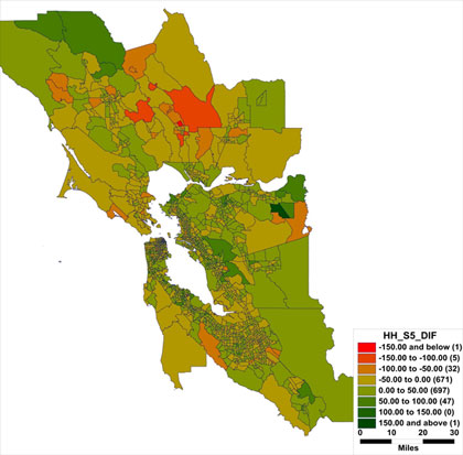
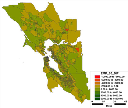
Figure 55 shows the reallocation of households for the most aggressive operations scenario (Scenario 5: ATDM and Signal Control) compared to the base. The area in and around the treatment areas received more growth at the expense of locations north of the Bay and on the extreme western edge of the area. Employment follows a similar pattern (Figure 56).
Figure 55. Map. Households.
(Source: Cambridge Systematics, Inc.)
Figure 56. Map. Employment.
(Source: Cambridge Systematics, Inc.)
The performance and emissions results are shown in Table 38. Regionally, base condition VMT increased 7.2 percent and VHT increased by 11.0 percent from 2010. As with the 2010 runs, VMT increases for each strategy over the base condition. The less aggressive operations strategies – signal control, ramp meters, and incident management – lead to a slight increases in emissions; the highest increase in CO2 is for ramp meters, which shows a one percent increase. For the aggressive ATDM strategies, the stronger effect on congestion (speeds) is enough to overcome the effect of increased VMT, resulting in reduced CO2 and hydrocarbon emissions.
An analysis of predicted trips in the model was undertaken to determine possible sources of the VMT increase. Table 39 shows the results comparing the base to Scenario 5 (ATDM + active signal control). The number of trips increased marginally (less than 0.2 percent) with the aggressive operations deployment. Average trip length increased by slightly more than 0.5 percent. The improved travel times are allowing travelers to make longer trips, thus increasing VMT for the operations deployment scenario.
Table 38. AM Peak Period performance results, 2015 MTC Model runs.
|
VHT |
VMT |
HC (grams) |
CO (grams) |
NOx (grams) |
CO2 (grams) |
County |
Highway Type |
| Base |
393,442 |
12,220,861 |
1,391,605 |
28,980,315 |
12,031,835 |
6,725,341,432 |
Remainder of Area |
Freeway |
| Base |
203,091 |
2,232,154 |
452,916 |
6,941,974 |
3,058,643 |
1,803,303,437 |
Remainder of Area |
Expressway |
| Base |
70,516 |
1,699,923 |
202,232 |
3,945,188 |
1,237,705 |
877,737,718 |
Remainder of Area |
Collector |
| Base |
212,841 |
5,803,389 |
616,269 |
12,567,232 |
3,825,586 |
2,788,290,112 |
Remainder of Area |
Arterial |
| Base |
344,807 |
9,017,018 |
1,146,229 |
21,833,457 |
8,916,526 |
5,168,631,628 |
Alameda/Contra Costa |
Freeway |
| Base |
53,693 |
447,662 |
105,937 |
1,400,605 |
850,541 |
401,278,728 |
Alameda/Contra Costa |
Expressway |
| Base |
43,328 |
1,000,917 |
122,043 |
2,361,566 |
723,370 |
523,529,941 |
Alameda/Contra Costa |
Collector |
| Base |
133,975 |
3,644,769 |
379,789 |
7,806,632 |
2,321,493 |
1,736,559,231 |
Alameda/Contra Costa |
Arterial |
| Base |
1,455,694 |
36,066,694 |
4,417,021 |
85,836,970 |
32,965,699 |
20,024,672,227 |
|
|
| S1: Active Signal Control |
401,189 |
12,235,788 |
1,407,291 |
29,108,165 |
12,111,596 |
6,771,984,953 |
Remainder of Area |
Freeway |
| S1: Active Signal Control |
210,244 |
2,233,149 |
458,109 |
6,987,465 |
3,083,708 |
1,821,727,703 |
Remainder of Area |
Expressway |
| S1: Active Signal Control |
70,211 |
1,692,140 |
200,330 |
3,914,745 |
1,229,353 |
870,927,062 |
Remainder of Area |
Collector |
| S1: Active Signal Control |
217,332 |
5,839,349 |
623,574 |
12,681,287 |
3,860,783 |
2,816,641,776 |
Remainder of Area |
Arterial |
| S1: Active Signal Control |
352,711 |
9,040,657 |
1,155,142 |
21,915,153 |
8,968,814 |
5,198,016,564 |
Alameda/Contra Costa |
Freeway |
| S1: Active Signal Control |
64,623 |
450,265 |
121,429 |
1,515,780 |
947,536 |
444,682,425 |
Alameda/Contra Costa |
Expressway |
| S1: Active Signal Control |
45,054 |
1,020,770 |
126,875 |
2,429,240 |
746,644 |
540,825,139 |
Alameda/Contra Costa |
Collector |
| S1: Active Signal Control |
129,173 |
3,674,163 |
372,257 |
7,733,173 |
2,313,768 |
1,715,854,911 |
Alameda/Contra Costa |
Arterial |
| S1: Active Signal Control |
1,490,537 |
36,186,280 |
4,465,007 |
86,285,007 |
33,262,202 |
20,180,660,532 |
|
|
| S1: Active Signal Control |
2.394% |
0.332% |
1.086% |
0.522% |
0.899% |
0.779% |
Compared to Base |
|
| S2: Ramp Meters |
412,555 |
12,257,958 |
1,430,489 |
29,340,667 |
12,213,152 |
6,838,410,969 |
Remainder of Area |
Freeway |
| S2: Ramp Meters |
217,915 |
2,241,396 |
472,475 |
7,108,349 |
3,169,096 |
1,864,040,915 |
Remainder of Area |
Expressway |
| S2: Ramp Meters |
69,972 |
1,707,420 |
201,162 |
3,938,447 |
1,239,070 |
875,662,292 |
Remainder of Area |
Collector |
| S2: Ramp Meters |
218,600 |
5,852,889 |
625,950 |
12,721,092 |
3,873,175 |
2,824,919,458 |
Remainder of Area |
Arterial |
| S2: Ramp Meters |
334,638 |
9,100,367 |
1,114,007 |
21,776,535 |
8,813,243 |
5,108,859,854 |
Alameda/Contra Costa |
Freeway |
| S2: Ramp Meters |
54,719 |
448,766 |
118,162 |
1,494,533 |
927,374 |
434,993,500 |
Alameda/Contra Costa |
Expressway |
| S2: Ramp Meters |
45,209 |
1,022,070 |
127,399 |
2,436,657 |
748,002 |
543,320,260 |
Alameda/Contra Costa |
Collector |
| S2: Ramp Meters |
133,636 |
3,659,023 |
380,477 |
7,829,279 |
2,327,038 |
1,740,989,328 |
Alameda/Contra Costa |
Arterial |
| S2: Ramp Meters |
1,487,244 |
36,289,890 |
4,470,120 |
86,645,558 |
33,310,149 |
20,231,196,576 |
|
|
| S2: Ramp Meters |
2.167% |
0.619% |
1.202% |
0.942% |
1.045% |
1.031% |
Compared to Base |
|
| S3: Incident Management |
420,623 |
12,284,568 |
1,452,433 |
29,553,596 |
12,309,064 |
6,906,416,238 |
Remainder of Area |
Freeway |
| S3: Incident Management |
220,438 |
2,234,450 |
472,066 |
7,099,075 |
3,163,275 |
1,860,908,081 |
Remainder of Area |
Expressway |
| S3: Incident Management |
71,097 |
1,718,773 |
203,593 |
3,978,073 |
1,249,326 |
885,263,311 |
Remainder of Area |
Collector |
| S3: Incident Management |
220,621 |
5,871,394 |
630,957 |
12,801,334 |
3,890,856 |
2,843,785,980 |
Remainder of Area |
Arterial |
| S3: Incident Management |
311,644 |
9,335,684 |
1,075,367 |
21,911,966 |
8,802,176 |
5,073,471,508 |
Alameda/Contra Costa |
Freeway |
| S3: Incident Management |
41,124 |
433,648 |
99,753 |
1,344,461 |
806,987 |
380,812,945 |
Alameda/Contra Costa |
Expressway |
| S3: Incident Management |
40,595 |
962,200 |
114,665 |
2,244,048 |
684,110 |
495,535,864 |
Alameda/Contra Costa |
Collector |
| S3: Incident Management |
124,718 |
3,520,726 |
358,209 |
7,441,855 |
2,215,235 |
1,651,602,071 |
Alameda/Contra Costa |
Arterial |
| S3: Incident Management |
1,450,860 |
36,361,443 |
4,407,042 |
86,374,408 |
33,121,030 |
20,097,795,998 |
|
|
| S3: Incident Management |
-0.332% |
0.817% |
-0.226% |
0.626% |
0.471% |
0.365% |
Compared to Base |
|
| S4: ATDM |
409,444 |
12,266,027 |
1,425,388 |
29,343,076 |
12,180,066 |
6,831,481,924 |
Remainder of Area |
Freeway |
| S4: ATDM |
217,300 |
2,236,041 |
471,569 |
7,101,660 |
3,161,113 |
1,861,368,136 |
Remainder of Area |
Expressway |
| S4: ATDM |
69,847 |
1,693,870 |
200,032 |
3,915,810 |
1,227,647 |
870,221,590 |
Remainder of Area |
Collector |
| S4: ATDM |
217,401 |
5,847,082 |
625,607 |
12,720,431 |
3,863,574 |
2,823,521,406 |
Remainder of Area |
Arterial |
| S4: ATDM |
295,085 |
9,605,683 |
1,054,067 |
22,270,882 |
8,907,319 |
5,089,339,035 |
Alameda/Contra Costa |
Freeway |
| S4: ATDM |
43,240 |
430,154 |
99,172 |
1,336,598 |
803,978 |
378,176,406 |
Alameda/Contra Costa |
Expressway |
| S4: ATDM |
39,468 |
949,106 |
112,658 |
2,208,121 |
672,798 |
487,438,437 |
Alameda/Contra Costa |
Collector |
| S4: ATDM |
120,181 |
3,435,328 |
345,476 |
7,215,036 |
2,148,394 |
1,599,164,007 |
Alameda/Contra Costa |
Arterial |
| S4: ATDM |
1,411,967 |
36,463,293 |
4,333,969 |
86,111,614 |
32,964,889 |
19,940,710,940 |
|
|
| S4: ATDM |
-3.004% |
1.100% |
-1.880% |
0.320% |
-0.002% |
-0.419% |
Compared to Base |
|
| S5: ATDM + Signal Control |
410,868 |
12,276,848 |
1,426,967 |
29,352,749 |
12,193,872 |
6,837,747,991 |
Remainder of Area |
Freeway |
| S5: ATDM + Signal Control |
219,959 |
2,247,907 |
474,433 |
7,139,118 |
3,176,150 |
1,871,409,334 |
Remainder of Area |
Expressway |
| S5: ATDM + Signal Control |
70,181 |
1,699,644 |
201,245 |
3,934,436 |
1,233,409 |
874,906,948 |
Remainder of Area |
Collector |
| S5: ATDM + Signal Control |
218,231 |
5,868,687 |
628,089 |
12,768,659 |
3,879,236 |
2,834,607,628 |
Remainder of Area |
Arterial |
| S5: ATDM + Signal Control |
298,693 |
9,626,802 |
1,058,957 |
22,306,865 |
8,934,607 |
5,110,098,537 |
Alameda/Contra Costa |
Freeway |
| S5: ATDM + Signal Control |
47,552 |
434,007 |
113,545 |
1,441,772 |
895,480 |
419,204,124 |
Alameda/Contra Costa |
Expressway |
| S5: ATDM + Signal Control |
39,577 |
939,996 |
111,495 |
2,185,333 |
666,320 |
482,448,682 |
Alameda/Contra Costa |
Collector |
| S5: ATDM + Signal Control |
115,999 |
3,451,111 |
338,955 |
7,149,167 |
2,137,742 |
1,579,924,272 |
Alameda/Contra Costa |
Arterial |
| S5: ATDM + Signal Control |
1,421,061 |
36,545,003 |
4,353,686 |
86,278,098 |
33,116,816 |
20,010,347,516 |
|
|
| S5: ATDM + Signal Control |
-2.379% |
1.326% |
-1.434% |
0.514% |
0.458% |
-0.072% |
Compared to Base |
|
| S6: Regional ATDM + Signal Control |
354,439 |
12,902,696 |
1,339,086 |
29,873,455 |
12,215,778 |
6,758,789,530 |
Remainder of Area |
Freeway |
| S6: Regional ATDM + Signal Control |
198,047 |
2,188,079 |
449,505 |
6,826,640 |
3,059,808 |
1,783,296,299 |
Remainder of Area |
Expressway |
| S6: Regional ATDM + Signal Control |
69,238 |
1,666,312 |
197,860 |
3,864,653 |
1,210,458 |
859,553,531 |
Remainder of Area |
Collector |
| S6: Regional ATDM + Signal Control |
200,271 |
5,664,682 |
589,402 |
12,115,961 |
3,702,167 |
2,681,332,522 |
Remainder of Area |
Arterial |
| S6: Regional ATDM + Signal Control |
302,019 |
9,644,383 |
1,064,017 |
22,388,120 |
8,959,102 |
5,127,966,003 |
Alameda/Contra Costa |
Freeway |
| S6: Regional ATDM + Signal Control |
47,307 |
436,356 |
113,753 |
1,446,595 |
897,455 |
420,327,610 |
Alameda/Contra Costa |
Expressway |
| S6: Regional ATDM + Signal Control |
39,593 |
940,007 |
111,573 |
2,186,386 |
666,067 |
482,674,153 |
Alameda/Contra Costa |
Collector |
| S6: Regional ATDM + Signal Control |
116,115 |
3,451,998 |
339,289 |
7,155,253 |
2,138,793 |
1,580,848,575 |
Alameda/Contra Costa |
Arterial |
| S6: Regional ATDM + Signal Control |
1,327,028 |
36,894,513 |
4,204,484 |
85,857,063 |
32,849,627 |
19,694,788,222 |
|
|
| S6: Regional ATDM + Signal Control |
-8.839% |
2.295% |
-4.812% |
0.023% |
-0.352% |
-1.647% |
Compared to Base |
|
Table 39. Bay Area regional trip making, 2015.
| County |
No. Trips – Base |
No. Trips – Scen. 5 |
No. Trips – Percent Change |
Average Trip Length (miles) – Base |
Average Trip Length (miles) – Scen. 5 |
Average Trip Length (miles) – Percent Change |
| San Francisco |
292,162 |
292,917 |
0.26% |
7.40 |
7.44 |
0.49% |
| San Mateo |
414,952 |
414,959 |
0.00% |
8.92 |
8.92 |
0.02% |
| Santa Clara |
1,112,990 |
1,113,110 |
0.01% |
8.41 |
8.44 |
0.28% |
| Alameda |
825,565 |
827,738 |
0.26% |
9.08 |
9.15 |
0.83% |
| Contra Costa |
586,928 |
588,966 |
0.35% |
9.42 |
9.49 |
0.78% |
| Solano |
235,684 |
236,438 |
0.32% |
10.82 |
10.91 |
0.82% |
| Napa |
79,934 |
79,885 |
-0.06% |
9.85 |
9.94 |
0.99% |
| Sonoma |
291,865 |
292,106 |
0.08% |
9.50 |
9.54 |
0.44% |
| Marin |
139,109 |
139,567 |
0.33% |
9.72 |
9.80 |
0.86% |
| External |
83,397 |
83,396 |
0.00% |
33.58 |
33.74 |
0.47% |
| TOTAL |
4,062,586 |
4,069,082 |
0.16% |
9.48 |
9.53 |
0.54% |
Note: “Scen. 5” is Scenario 5, ATDM + active signal control.
As shown in Table 38, an additional scenario was created for the 2015 runs: Scenario 6, deployment of ATDM and active signal control on all freeways and arterials in the nine county region, respectively. This run is not “complete” in the sense that there was no 2010 run on which to base land use changes. (It used land use input from Scenario 5.) It was created to see what effect full operations deployment might have. If full deployment had been achieved in 2010, would population and employment be shifted around as shown above? Our guess is that most of the shifting would be from outside the region, as the travel time improvements would be ubiquitous within the region, thereby not giving any location an advantage in terms of accessibility. Still, the regional deployment scenario results in a 2.3 percent increase in VMT, an 8.8 percent decrease in VHT, and a decrease in CO2 emissions of 1.6 percent. The VMT increase is double what it is for deployment in only Alameda and Contra Costa counties, indicating that the improved regional travel times are having an effect on regional traveler behavior. Despite the VMT increase, regional deployment of aggressive operations is seen as having a positive impact on CO2 emissions.
The above results may be dependent on the nature of congestion in the network, which is severe. To test this, we took the model runs from above and postprocessed to get hourly speeds and emissions, but without the 30 percent increase in the v/c ratio.
I-15 Traffic Simulation Analysis with Updated Demand
The final step in the analysis was to use the long-term demand shifts obtained in the regional modeling analysis as input to the I-15 traffic simulation framework to get more refined emissions estimates. Ideally, this task would be done simultaneously with the land use/demand modeling step, but as previously noted, the complete modeling framework for doing so does not exist.
Several scenarios from the original I-15 runs were selected for conducting the comparisons. Table 40 shows the scenarios and the demand changes that were used. The demand changes are based on the data in Table 36. It should be noted that, as shown in the MTC model runs, there will be demand changes beyond the small subarea covered by the I-15 test network.
Table 40. Demand changes applied to I-15 scenarios.
| Scenario |
Features |
Demand Changes |
| A |
Ramp metering |
+1.0% major arterials |
| E |
Ramp metering
Minor Incident withTIM
Traveler Information |
+3.5% I-15 SB
-3.5% major arterials |
| E2 |
Ramp metering
Minor Incident withTIM |
+3.5% I-15 SB
-3.5% major arterials |
| G |
Ramp metering
Active signal control |
+2.0% I-15 SB
+1.0% major arterials |
| H |
Ramp metering
Active signal control
Traveler Information |
+2.5% I-15 SB
+1.5% major arterials |
Modifying demands in the traffic simulation model is an indirect task. VMT is “emergent” from the model; it is not an input. Rather, VMT is a result from the loading of trip tables onto the network. Therefore, the trip tables were modified using the following steps. Vehicles moving in the southbound direction of I-15 and on Pomerado Road were identified and their paths were traced backwards and forward to identify those origins and destinations in the trip matrix that assign vehicles to the SB direction of I-15; this is known as “select link analysis. After the select link analysis was performed, the flow of those O-D pairs was increased or decreased in the trip matrix that take I-15 SB or Pomerado Road in the base-year model.
The results are shown in Tables 41 and 42. The scenarios tagged with “_Incr” represent the new simulation runs with the demand changes. The original runs also are shown for comparison. The base condition for the nonincident scenarios is Scenario F, as before (no operations treatments deployed.) For the incident scenarios, the base condition for is Scenario D for Scenario E and E_Incr and Scenario D2 for Scenario E2 and E2_Incr.
Overall, the increased demand scenarios for nonincident conditions still show a benefit (decrease in CO2 emissions), albeit smaller than for original scenarios. This result may be an artifact of trying to get VMT increases on the network by modifying the trip table – trips will be redistributed to some degree by the model. Still, this is a representation of how the system will “handle” additional demand, much better than trying to force the target VMT onto the desired roadways. These results are similar to those obtained with the MTC travel model for the high order MTC Scenarios S4 through S6 which represent bundles of strategies similar to what is done for the I-15 tests.
As with the original demand runs, the effect of adding traveler information is likely problematic due to how the model simulates it – the “G” scenarios outperform the “H” scenarios even though the latter have traveler information added. The “H” scenarios have a higher VMT, indicating more circuitous routing. As shown back in Table 29, the overall system speed also is higher for the “H” scenarios. These conditions would lead to increased emissions for the “H” versus the “G” scenarios, assuming the internal algorithm is acting reasonably. Unfortunately, there is no way to validate the reasonableness; research on how travelers react to information is lacking.
However, the ability to replicate the network VMT changes noted in the MTC runs by adjusting the TransModeler trip table proved to be very difficult. In all cases, adjusting the origin-destination flows by the percentages in Table 40 resulted in less VMT than observed in the MTC model. This may reflect the differences in assignment procedures between the travel demand and simulation model. It also points out the problems associated with trying to integrate two separate modeling frameworks. In any event, because the VMT gains are not as large as originally planned, despite multiple attempts to adjust the trip table, the emission reductions in Tables 41 and 42 are most probably overestimated. Because the gains are still relatively large, though, we would expect that some reductions would still remain, or that the change would be so small that the net effect would be neutral.
The incident scenarios exhibit a similar pattern, but with Scenario E_Incr showing a slight increase (half a percent) in CO2 emissions. These results are in contrast to the MTC results for incident management which showed an increase in CO2 emissions. However, the MTC network was for a generalized condition – the capacity was increased to reflect the cumulative annual effect of incident management (seven percent) rather than modeling a specific incident, as is done for I-15. In the I-15 case, the net capacity equivalent increase is much larger. The MTC model showed that when capacity is only increased marginally (e.g., Scenarios S1 through S3), the effect of the increased demand causes emissions to increase, whereas when it is larger, the effect of the improvement absorbs the increased demand. This may in fact be a function of the volume-delay relationship used in the MTC model.
Table 41. I-15 Traffic simulation results with increased demand, nonincident scenarios.
| 6:00 a.m. to 9:00 a.m. – Route |
6:00 a.m. to 9:00 a.m. – Scenario |
VMT |
Emissions – CO2 |
Emissions – CO2 Relative to Base |
Emissions – CO |
Emissions – HC |
Emissions – NOx |
| Black Mountain Expressway |
base |
10,352 |
6,765,509 |
|
95,438 |
2,806 |
15,305 |
| Black Mountain Expressway |
scenario_A |
9,594 |
7,044,845 |
4.13% |
93,865 |
2,994 |
15,448 |
| Black Mountain Expressway |
scenario_A_Incr |
10,742 |
7,887,795 |
16.59% |
91,975 |
2,674 |
15,010 |
| Black Mountain Expressway |
scenario_G |
10,812 |
6,638,842 |
-1.87% |
95,103 |
2,745 |
15,306 |
| Black Mountain Expressway |
scenario_G_Incr |
10,594 |
6,414,223 |
-5.19% |
93,105 |
2,647 |
15,080 |
| Black Mountain Expressway |
scenario_H |
10,452 |
6,626,596 |
-2.05% |
94,349 |
2,776 |
15,424 |
| Black Mountain Expressway |
scenario_H_Incr |
10,926 |
6,975,757 |
3.11% |
100,259 |
2,952 |
15,771 |
| Carmel Mountain Expressway |
base |
4,816 |
2,886,183 |
|
51,597 |
1,228 |
6,925 |
| Carmel Mountain Expressway |
scenario_A |
4,309 |
2,907,180 |
0.73% |
51,873 |
1,238 |
6,924 |
| Carmel Mountain Expressway |
scenario_A_Incr |
4,758 |
2,862,494 |
-0.82% |
51,480 |
1,220 |
6,885 |
| Carmel Mountain Expressway |
scenario_G |
4,803 |
2,723,066 |
-5.65% |
43,797 |
1,213 |
5,929 |
| Carmel Mountain Expressway |
scenario_G_Incr |
4,723 |
3,337,988 |
15.65% |
57,768 |
1,647 |
7,957 |
| Carmel Mountain Expressway |
scenario_H |
4,882 |
2,937,542 |
1.78% |
52,440 |
1,250 |
7,069 |
| Carmel Mountain Expressway |
scenario_H_Incr |
4,912 |
3,000,084 |
3.95% |
60,795 |
1,788 |
8,612 |
| I-15 NB |
base |
297,336 |
109,295,860 |
|
1,121,967 |
33,210 |
250,478 |
| I-15 NB |
scenario_A |
289,513 |
104,558,162 |
-4.33% |
1,058,182 |
31,576 |
239,653 |
| I-15 NB |
scenario_A_Incr |
278,534 |
101,954,652 |
-6.72% |
1,026,712 |
30,888 |
231,951 |
| I-15 NB |
scenario_G |
282,783 |
104,808,784 |
-4.11% |
1,066,312 |
31,960 |
239,578 |
| I-15 NB |
scenario_G_Incr |
282,195 |
105,752,063 |
-3.24% |
1,019,619 |
30,777 |
231,155 |
| I-15 NB |
scenario_H |
292,487 |
108,973,584 |
-0.29% |
1,127,518 |
33,546 |
247,793 |
| I-15 NB |
scenario_H_Incr |
295,704 |
110,172,293 |
0.80% |
1,128,082 |
33,848 |
250,221 |
| I-15 SB |
base |
420,698 |
217,218,389 |
|
1,954,660 |
81,830 |
427,100 |
| I-15 SB |
scenario_A |
435,030 |
213,456,303 |
-1.73% |
1,867,652 |
80,948 |
413,619 |
| I-15 SB |
scenario_A_Incr |
432,522 |
211,748,653 |
-2.52% |
1,845,240 |
80,381 |
411,965 |
| I-15 SB |
scenario_G |
421,320 |
188,302,302 |
-13.31% |
1,823,462 |
65,871 |
398,333 |
| I-15 SB |
scenario_G_Incr |
427,786 |
190,829,990 |
-12.15% |
1,765,743 |
60,263 |
387,891 |
| I-15 SB |
scenario_H |
418,841 |
203,885,665 |
-6.14% |
1,910,878 |
74,227 |
417,795 |
| I-15 SB |
scenario_H_Incr |
423,449 |
206,128,407 |
-5.11% |
1,911,833 |
75,224 |
421,555 |
| I-15 SB |
scenario_F |
420,698 |
217,218,389 |
|
1,954,660 |
81,830 |
427,100 |
| Other Freeways/Expressways and Major Arterials |
base |
90,458 |
58,316,447 |
|
753,250 |
25,153 |
123,247 |
| Other Freeways/Expressways and Major Arterials |
scenario_A |
81,497 |
58,168,884 |
-0.25% |
747,604 |
25,171 |
122,648 |
| Other Freeways/Expressways and Major Arterials |
scenario_A_Incr |
92,853 |
59,216,202 |
1.54% |
727,231 |
22,357 |
116,213 |
| Other Freeways/Expressways and Major Arterials |
scenario_G |
93,510 |
56,799,069 |
-2.60% |
756,325 |
24,310 |
121,797 |
| Other Freeways/Expressways and Major Arterials |
scenario_G_Incr |
92,291 |
53,693,987 |
-7.93% |
734,386 |
22,746 |
116,776 |
| Other Freeways/Expressways and Major Arterials |
scenario_H |
94,426 |
56,399,555 |
-3.29% |
751,274 |
24,110 |
121,424 |
| Other Freeways/Expressways and Major Arterials |
scenario_H_Incr |
92,149 |
55,407,653 |
-4.99% |
745,615 |
23,817 |
118,645 |
| Pomerado Road |
base |
31,581 |
21,129,853 |
|
245,072 |
9,163 |
43,000 |
| Pomerado Road |
scenario_A |
28,106 |
21,551,594 |
2.00% |
244,971 |
9,468 |
42,992 |
| Pomerado Road |
scenario_A_Incr |
33,966 |
26,045,133 |
23.26% |
293,087 |
11,293 |
51,540 |
| Pomerado Road |
scenario_G |
32,921 |
17,457,167 |
-17.38% |
231,456 |
7,224 |
37,600 |
| Pomerado Road |
scenario_G_Incr |
33,804 |
16,755,750 |
-20.70% |
224,404 |
6,877 |
36,466 |
| Pomerado Road |
scenario_H |
35,003 |
16,982,701 |
-19.63% |
231,020 |
6,969 |
37,345 |
| Pomerado Road |
scenario_H_Incr |
36,480 |
18,857,549 |
-10.75% |
247,990 |
7,818 |
40,789 |
| Total, All Highways |
base |
855,241 |
415,612,241 |
|
4,221,984 |
153,390 |
866,055 |
| Total, All Highways |
scenario_A |
848,049 |
407,686,968 |
-1.91% |
4,064,147 |
151,395 |
841,284 |
| Total, All Highways |
scenario_A_Incr |
853,375 |
409,714,929 |
-1.42% |
4,035,726 |
148,814 |
833,563 |
| Total, All Highways |
scenario_G |
846,149 |
376,729,230 |
-9.36% |
4,016,455 |
133,323 |
818,543 |
| Total, All Highways |
scenario_G_Incr |
851,392 |
376,784,001 |
-9.34% |
3,895,024 |
124,957 |
795,326 |
| Total, All Highways |
scenario_H |
856,091 |
395,805,643 |
-4.77% |
4,167,478 |
142,879 |
846,849 |
| Total, All Highways |
scenario_H_Incr |
863,620 |
400,541,744 |
-3.63% |
4,194,575 |
145,446 |
855,592 |
Note: VMT for the increased demand scenarios were lower than the target values developed by the MTC regional model; see text for explanation
Table 42. I-15 Traffic simulation results with increased demand, incident scenarios
| 6:00 a.m. to 9:00 a.m. – Route |
6:00 a.m. to 9:00 a.m. – Scenario |
VMT |
Emissions – CO2 |
Emissions – CO2 Relative to Base |
Emissions – CO |
Emissions – HC |
Emissions – NOx |
| Black Mountain Expwy |
scenario_D |
10,510 |
6,612,747 |
|
93,907 |
2,776 |
15,239 |
| Black Mountain Expwy |
scenario_D2 |
10,352 |
6,630,833 |
|
94,364 |
2,731 |
15,132 |
| Black Mountain Expwy |
scenario_E |
11,173 |
7,012,707 |
6.05% |
99,367 |
2,966 |
15,830 |
| Black Mountain Expwy |
scenario_E_Incr |
10,782 |
6,951,142 |
5.12% |
98,729 |
2,885 |
15,913 |
| Black Mountain Expwy |
scenario_E2 |
11,159 |
7,253,787 |
9.39% |
100,984 |
3,053 |
16,385 |
| Black Mountain Expwy |
scenario_E2_Incr |
10,982 |
6,798,387 |
2.53% |
95,149 |
2,837 |
15,441 |
| Carmel Mountain Expwy |
scenario_D |
4,917 |
2,954,354 |
|
52,713 |
1,256 |
7,036 |
| Carmel Mountain Expwy |
scenario_D2 |
4,784 |
2,859,546 |
|
51,033 |
1,217 |
6,846 |
| Carmel Mountain Expwy |
scenario_E |
4,916 |
2,962,320 |
0.27% |
52,780 |
1,261 |
7,094 |
| Carmel Mountain Expwy |
scenario_E_Incr |
4,795 |
3,600,557 |
21.87% |
64,111 |
1,535 |
8,587 |
| Carmel Mountain Expwy |
scenario_E2 |
4,970 |
3,054,455 |
6.82% |
54,347 |
1,304 |
7,304 |
| Carmel Mountain Expwy |
scenario_E2_Incr |
4,859 |
2,915,883 |
1.97% |
52,162 |
1,243 |
6,955 |
| Black Mountain Expwy |
scenario_D |
10,510 |
6,612,747 |
|
93,907 |
2,776 |
15,239 |
| I-15 NB |
scenario_D |
293,290 |
108,978,872 |
|
1,120,279 |
33,379 |
249,102 |
| I-15 NB |
scenario_D2 |
297,320 |
109,779,783 |
|
1,129,933 |
33,453 |
252,169 |
| I-15 NB |
scenario_E |
286,463 |
105,920,289 |
-2.81% |
1,084,187 |
32,254 |
242,596 |
| I-15 NB |
scenario_E_Incr |
281,058 |
105,558,896 |
-3.14% |
1,063,220 |
31,957 |
241,460 |
| I-15 NB |
scenario_E2 |
286,324 |
106,184,196 |
-3.28% |
1,085,910 |
32,348 |
243,117 |
| I-15 NB |
scenario_E2_Incr |
278,526 |
103,421,845 |
-5.79% |
1,057,423 |
31,706 |
235,818 |
| I-15 SB |
scenario_D |
416,604 |
208,120,832 |
|
1,918,518 |
76,583 |
419,330 |
| I-15 SB |
scenario_D2 |
414,197 |
211,701,360 |
|
1,929,704 |
80,855 |
410,968 |
| I-15 SB |
scenario_E |
430,183 |
182,615,160 |
-12.26% |
1,831,966 |
62,389 |
397,495 |
| I-15 SB |
scenario_E_Incr |
431,949 |
209,535,741 |
0.68% |
1,905,049 |
76,875 |
421,994 |
| I-15 SB |
scenario_E2 |
410,096 |
186,308,356 |
-11.99% |
1,862,559 |
64,489 |
403,501 |
| I-15 SB |
scenario_E2_Incr |
431,949 |
211,652,264 |
-0.02% |
1,939,376 |
77,573 |
427,985 |
| Pomerado Rd |
scenario_D |
34,917 |
17,214,891 |
|
231,881 |
7,049 |
37,527 |
| Pomerado Rd |
scenario_D2 |
31,381 |
21,087,603 |
|
243,132 |
9,221 |
42,131 |
| Pomerado Rd |
scenario_E |
38,660 |
18,930,927 |
9.97% |
251,358 |
7,707 |
41,510 |
| Pomerado Rd |
scenario_E_Incr |
33,226 |
16,979,567 |
-1.37% |
227,540 |
6,998 |
36,845 |
| Pomerado Rd |
scenario_E2 |
38,750 |
18,952,848 |
-10.12% |
251,671 |
7,727 |
41,691 |
| Pomerado Rd |
scenario_E2_Incr |
34,473 |
17,251,432 |
-18.19% |
231,422 |
7,153 |
37,424 |
| Total, All Highways |
scenario_D |
854,724 |
398,780,996 |
|
4,161,531 |
144,340 |
847,496 |
| Total, All Highways |
scenario_D2 |
847,565 |
409,479,626 |
|
4,192,276 |
152,289 |
848,306 |
| Total, All Highways |
scenario_E |
870,298 |
373,213,303 |
-6.41% |
4,084,703 |
130,084 |
826,647 |
| Total, All Highways |
scenario_E_Incr |
861,320 |
400,813,116 |
0.51% |
4,146,083 |
144,830 |
851,656 |
| Total, All Highways |
scenario_E2 |
850,810 |
379,940,855 |
-7.21% |
4,142,905 |
133,500 |
838,856 |
| Total, All Highways |
scenario_E2_Incr |
855,124 |
396,178,359 |
-3.25% |
4,116,733 |
143,475 |
841,704 |
Note: VMT for the increased demand scenarios were lower than the target values developed by the MTC regional model; see text for explanation.
You may need the Adobe® Reader® to view the PDFs on this page.
|



