Travel and Emissions Impacts of Highway Operations Strategies

Chapter 4. Reliability-Land Use

Introduction

The objective for this component of the research project is to develop a methodology to evaluate the long-term effects of operations strategies. We interpret long-term effects to be those that are beyond the time-scale of within-day travel decisions, and in the time-scale of land use impacts such as real estate prices and rents, location choices of households, workers and firms, and real estate development outcomes.

Agencies considering the implementation of alternative operations strategies to improve reliability and reduce congestion are unlikely to take into account that there might be impacts on land use. This has two implications. First, there may be long-term benefits in terms of property value appreciation, economic development, and resulting tax revenues that have been overlooked in decision-making about system improvements that target improvements in reliability. If so, this would imply an underestimation of the benefits of such projects. Second, these land use impacts may impact travel patterns in ways that induce more travel and undermine at least part of the gains in reliability or congestion. The broader literature on induced demand suggests that transportation system interventions that improve travel time not only result in short-term responses by travelers to shift modes, times of travel and routes (Downs, 2004), but also include longer-term influence on land use outcomes that further affect travel demand (Waddell, Ulfarsson, Franklin, and Lobb, 2007; Noland, 2001). This literature has not explored, however, whether improvements in travel-time reliability might generate long-term impacts on real estate markets.

Even the casual observer would likely agree that unreliable travel time to work is problematic, and a growing body of research has begun to measure the degree to which travelers value travel-time reliability by analyzing their route or mode choices (Bates, Polak, Jones, and Cook, 2001; Lam and Small, 2001; Ettema, Tamminga, Timmermans, and Arentze, 2005; Nam, Park, and Khamkongkhun, 2005; Brownstone and Small, 2005; Small, Winston, and Yan, 2005; van Lint, van Zuylen, and Tu, 2008; Li, Hensher and Rose, 2010; Fosgerau and Karlström, 2010). To our knowledge, however, no one has yet addressed the question of whether travel-time reliability has longer-term effects beyond daily travel decisions, by influencing real estate market outcomes. Is travel-time reliability valued enough by individuals, households, and firms to be capitalized into higher real estate prices and rents in locations with more reliable accessibility? Does reliability have enough value to influence long-term choices of households or firms regarding where they rent or purchase real estate? These are the questions explored in this research.

The theoretical grounding for this research draws on urban economics and on the geography of transportation. The role of accessibility in shaping urban form and location choices has been central to the development of this literature, from the early conceptualization and measurement of accessibility (Hansen, 1959) and the emergence of urban land use models that explained the capitalization of accessibility into land values via bid-rent theory (Alonso, 1960; Muth, 1961). Recent research on the impact of accessibility has been mixed, with some scholars questioning the relative importance of accessibility in modern polycentric cities with complex household choices regarding work and residence locations (Giuliano, 2004; Gordon and Richardson, 1997), while others have explored the empirical role of accessibility at localized and regional scales on land use outcomes such as residential location choices, finding that both remain significant when carefully measured (Waddell and Nourzad, 2002; Lee, Waddell, Wang and Pendyala, 2010).

Core theoretical building blocks for this research include bid-rent theory, put forward in the early development of urban economics as a field (Alonso, 1960; Muth, 1961), and hedonic regression, a methodology to estimate the implicit prices of amenities in bundled goods, such as housing (Rosen, 1974). Combining these two building blocks, extensive research has been done to analyze how locational amenities such as accessibility are capitalized into residential property values (Nelson, 1977; Edmonds, 1983; Waddell, Berry and Hoch, 1993; Waddell and Nourzad, 2002; Lee et al., 2010), as well as apartment rents (Hoch and Waddell, 1993), and office rents (Rosen, 1984; Mills, 1992).

The logic behind this theoretical approach is quite straightforward: agents that value-specific amenities such as travel time savings will bid more in terms of rent or purchase price at those locations that have higher values of such amenities, and in so doing, they are more likely to outbid other agents for the real estate at those sites. A further consequence of this logic is that higher competition for advantageous sites results in higher land values and subsequently translates to a higher development intensity on such sites, as a result of substitution from increasingly expensive land costs to relatively less expensive capital costs in the form of taller buildings through capital-land substitution.

A final theoretical building block for this work is that of discrete choice modeling of location choice, pioneered by Daniel McFadden in the context of residential location choices (McFadden, 1978), and extended to become a foundation of most empirical research on travel demand and a critical component of operational travel demand models (Ben-Akiva and Lerman, 1987; Train, 2009). Discrete choice methods have permitted examination of the tradeoffs that households make between the structural and contextual amenities of a house, its price, and its accessibility. It therefore provides a direct approach to measuring the value of reliability and its influence on location demand. Extensive prior work on modeling residential location choices (Waddell, 1997; Waddell, 2000; Waddell, 2007; Waddell, Wang, Charlton, and Olsen, 2010), in addition to related research on modeling the location choices of firms (business location) (Shukla and Waddell, 1991; Waddell and Shukla, 1993; Waddell and Shukld, 1993; Waddell and Ulfarsson, 2003), and the workplace choices of workers (Wang, Waddell, and Outwater, 2011), provide a strong foundation for the empirical component of this research.

Methodology

In this section we describe our research approach for developing a quantitative basis for assessing the long-term effects of operations strategies. We set aside the details of the operations strategies, and focus on the outcomes of operations that could impact land use: mean travel time and its reliability. Further, we particularly focus on how travel-time reliability impacts land use, since this has not been explored previously.

We develop an application platform for simulating the effects of alternative interventions that change patterns of travel-time reliability. For this application component, we have adapted UrbanSim, an operational land use model system that has been connected to a variety of four-step and activity-based travel models in addition to dynamic assignment models (Waddell, 2011; Waddell, 2002; Waddell et al., 2007; Waddell et al., 2010; Pendyala, Konduri, Chiu, Hickman, Noh, Waddell, Wang, You and Gardner, 2012). Our approach to this task was to add travel-time reliability into UrbanSim models of residential location choice, business location choice, workplace choice, and real estate rents and prices in order to simulate their impacts across the full study area. The objective is to provide a generic capability to address long-term land use impacts of operations improvements by allowing them to be tested in a land use modeling platform that has been extended to address reliability-enhanced accessibility measures.

Study Area and Data

Our study area is the San Francisco Bay area, consisting of nine counties for which the Metropolitan Transportation Commission and the Association of Bay Area Governments develop the regional transportation plan and sustainable communities strategies. For this region, we compiled extensive land use and travel time data for the development of both the empirical research component and for the large-scale application and testing of the approach.

Figure 24. Map. San Francisco Bay Area.

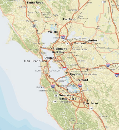
(Source: Red Hat, Inc.)

We developed an extensive database for the San Francisco Bay Area containing the following data elements to reflect the real estate, business, and demographic environment, as well as transportation networks and observed travel time distributions:

• Parcels, including attributes such as lot size, land use, and property value.
• Buildings, including building type, square footage, stories, residential units.
• Sales Transactions, including sales of condominiums and single-family homes.
• Rents, including apartments, offices from CoStar, Craig’s List, and other sources.
• Businesses from the National Establishment Time Series (NETS).
• Household Travel Survey from Bay Area Transportation Survey (BATS).
• Synthetic Population from the Metropolitan Transportation Commission, including households and persons.
• Streets from OpenStreetMap.
• Travel Model Network from the Metropolitan Transportation Commission.
• PeMS Travel Times from the Caltrans Performance Measurement System (PeMS) real-time traffic data on highways in California.

Travel-time reliability is intuitively linked to the width of the travel-time distribution. The reliability is quantified in various ways, including statistical range measures, buffer measures, and tardy trip indicators such as the misery index (Lomax, Schrank, Turner, and Margiotta, 2003). Comparing the 80^th and 50^th percentile travel times (Small et al., 2005) presents a nonparametric reliability metric with units of travel time.

Our travel time data for this project is drawn from the Caltrans Performance Measurement System (PeMS) real-time traffic data on highways in California. The average travel time and volume on each link in the network was computed at 30-minute intervals. Further processing was done to generate a set of quantile metrics: the volumes and speeds associated with the minimum, 20^th, 50^th (median), and 80^th percentile on each link for the morning peak period on a daily basis. Only weekdays were used in this analysis.

Research Hypotheses

The empirical research objectives of this project are the following, based on hypothesized influences that reliability of travel time could influence different long-term land use outcomes. Our first hypothesis is that, after controlling for accessibility and other factors, rents, and transactions prices for real estate will be higher in locations that have relatively higher travel-time reliability, consistent with the capitalization of the amenity value of reliability into property values and rents. In short, if reliability is valued by households or firms, they will be willing to pay more in rent or purchase price for real estate in locations that are more reliably accessible, all else being equal. And as a result of competition for real estate, drawing on bid-rent theory, we should see higher market rents and transactions prices in locations with more reliable access. This hypothesis can be tested using hedonic regression models of rents and transactions prices to estimate the implicit price of reliability (Rosen, 1974).

The approach to estimating implicit prices using hedonic regression is widely used in the literature, and provides a reduced-form approach that enables assessment of overall market impacts of reliability. A complementary strategy allows us to extend this research to a more structural approach to test two further hypotheses. If we find that either residential rents and prices, or nonresidential rents, are higher in areas with higher reliability, then we can further explore the structural origins of this market effect. It could alternatively arise from influences on the supply side or the demand side of the real estate market. It is in our view more likely that travel-time reliability would influence real estate demand, since prior research has demonstrated that travelers value travel-time reliability enough to influence their mode and route choices (Bates et al., 2001; Lam and Small, 2001; Ettema et al., 2005; Nam et al., 2005; Small et al., 2005; van Lint et al., 2008; Li et al., 2010). We know of no research that has suggested that travel-time reliability could influence the cost or feasibility of real estate development, and it seems unlikely that there should be such an effect. Consequently, our second and third hypotheses focus on the structural origins of any price effects we find by examining whether household and firm location choices are influenced by travel-time reliability.

• Hypothesis 1: Locations with more reliable accessibility have higher real estate prices and rents, capitalizing the amenity value of travel-time reliability.
• Hypothesis 2: Household residential location choices reveal a preference for residential locations that have more reliable accessibility.
• Hypothesis 3: Business location choices reveal a preference for establishment locations that have more reliable accessibility.

To evaluate the influence of travel time on long-term outcomes, we used the distribution of travel times as the basis for quantifying travel-time reliability. Prior work has examined simple measures such as standard deviations or other measures of variance, some research has pointed out limitations of this approach (van Lint et al., 2008). We focus in particular on the testing of accessibility using a median travel time value, and of reliability using the difference between the accessibility using the median travel time and the value using the 80^th percentile of the travel time distribution.

Real Estate Prices and Rents

Real estate prices and rents provide indicators of the balance between demand and supply of land at different locations and with different land use types, and of the relative market valuations for attributes of housing, nonresidential space, and location. This role is important to the rationing of land and buildings to consumers based on preferences and ability to pay, as a reflection of the operation of actual real estate markets. Since prices enter the location choice utility functions for jobs and households, an adjustment in prices will alter location preferences. All else being equal, this will in turn cause higher price alternatives to become more likely to be chosen by occupants who have lower price elasticity of demand. Similarly, any adjustment in land prices alters the preferences of developers to build new construction by type of space, and the density of the construction.

Real estate prices are modeled using a hedonic regression of the log-transformed property value per square foot on attributes of the parcel and its environment, including land use mix, density of development, proximity of highways and other infrastructure, land use plan or zoning constraints, and neighborhood effects. The hedonic regression equation encapsulates interactions between market demand and supply, revealing an envelope of implicit valuations for location and structural characteristics (DiPasquale and Wheaton, 1996). The model was estimated from sales transactions and observed rents from MLS and CoStar data sources, using Ordinary Least Squares (OLS), using a standard semi-log specification in which the dependent variable is log-transformed:

Figure 25. Equation. Log(Pi).

where i indexes locations defined as nodes on the local street network and the parcels associated with them, and E is the error term. Prices and rents by street node are computed as the average by building type among the parcels assigned to their nearest street node.

The independent variables influencing land prices can be organized into site characteristics, regional accessibility, and urban-design scale effects, as shown in Table 18.

Table 18. Variables in the hedonic regressions.

	Variable	Description
Site Characteristics	Number of stories (nonresidential)	Number of stories in building square feet of rentable building
Site Characteristics	Rentable building area	Log of square footage of building for nonresidential property
Site Characteristics	Square footage of the unit	Log of square footage of the unit for residential units
Site Characteristics	Lot size	Log of square footage of the lot
Site Characteristics	Historic	Indicator for construction before 1940
Site Characteristics	New	Indicator for construction after 1980
Regional Accessibility	Median accessibility	Log of number of jobs accessible within 30 minutes using median travel time
Regional Accessibility	Unreliability of accessibility	Log of (Accessibility using median travel time minus accessibility at 80th percentile travel time)
Neighborhood Characteristics	Average household income	Average income at the intersection

Household and Firm Location Choices

In order to empirically test our second and third hypotheses, we develop multinomial logit models of household residential location choice and establishment location choice. Our approach draws on the path breaking approach to modeling individual actions using discrete choice models pioneered by Daniel McFadden on Random Utility Maximization theory (McFadden, 1974; McFadden, 1981). This approach derives a model of the probability of choosing among a set of available alternatives based on the characteristics of the chooser and the attributes of the alternative, and proportional to the relative utility that the alternatives generate for the chooser. Maximum likelihood and simulated maximum likelihood methods have been developed to estimate the parameters of these choice models from data on revealed or stated-preferences, using a wide range of structural specifications (see Train, 2003). Early application of these models were principally in the transportation field such as mode choice, but also included work on residential location choices (Quigley, 1976; Lerman, 1977; McFadden, 1978), and on residential mobility (Clark and Lierop, 1986).

Consider a model of households choosing among alternative locations in the housing market, which we index by i. For each agent, we assume that each alternative i has associated with it a utility U_i that can be separated into a systematic part, V_i, and a random part, E_i:

Figure 26. Equation. U subscript i.

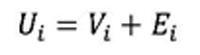
(Source: Waddell, 2000.)

where Vi = β·∙ x_i is a linear-in-parameters function, β is a vector of k estimable coefficients, x_i is a vector of observed, exogenous, independent alternative-specific variables that may be interacted with the characteristics of the agent making the choice, and E_i is an unobserved random term. Assuming the unobserved term in (2) to be distributed with a Gumbel distribution leads to the widely used multinomial logit model (McFadden, 1974; McFadden, 1981):

Figure 27. Equation. P subscript i.

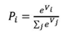
(Source: McFadden, 1974; McFadden, 1981.)

where j is an index over all possible alternatives. The estimable coefficients of (3), β, are estimated with the method of maximum likelihood (see for example Greene, 2002). The components of x_i are listed in Tables 19 and 20.

Table 19. Variables in the residential location choice models.

	Variable	Description
Renter Model	Monthly rent	Monthly rent per unit
Renter Model	Number of units	Number of residential units at the intersection
Renter Model	Node renters	Number of renters at the intersection
Renter Model	Area renters	Number of renters in the area
Sales Model	Sales price	Sales price per unit at the intersection
Sales Model	Average income	Average income at the intersection
Sales Model	Number of units	Number of residential units at the intersection
Renter and Sales Models	Median accessibility	Log of number of jobs accessible within 30 minutes using median travel time
Renter and Sales Models	Unreliability of accessibility	Log of (Accessibility at median travel time minus Accessibility at 80th percentile travel time)

Table 20. Variables in the nonresidential location choice models.

	Variable	Description
Area Attributes	Area	Square footage at intersection
Area Attributes	Percent retail	Percent of local establishments in retail
Area Attributes	Percent industrial	Percent of local establishments in industrial
Property Attributes	Rent	Square footage-weighted yearly rent
Regional Accessibility	Median accessibility	Log of number of jobs accessible within 30 minutes using median travel time
Regional Accessibility	Unreliability of Accessibility	Log of (Accessibility at median travel time minus Accessibility at 80th percentile travel time)

Estimation Results

Our empirical study of the effects of accessibility and its reliability proceeds in two parts. The first part examines the degree to which we can identify the implicit prices of reliability, which we measure as the access to jobs within 30 minutes travel time at the median of the travel time distribution, minus the same measure of accessibility computed using the 80^th percentile travel time. The more unreliable the travel time is, the greater is the deviation from the median travel time, and the larger is the gap between accessibility on a typical day (the median) and on what could be considered the average worst day of the week (the 80^th percentile). Areas that have unreliable freeways around them will have much lower accessibility to jobs on those 80^th percentile days than they do on the median days.

Hedonic Regression of Real Estate Prices and Rents

We measure the degree to which this unreliability in accessibility is capitalized into rents and property values, using hedonic regression, for each property type. Rents and prices are aggregated by parcel to the nearest street node, and these nodes are the unit of analysis for the hedonic regression. Prices and rents are log-transformed.

Our estimation results strongly support our first hypothesis that locations with more reliable accessibility have higher real estate prices and rents, capitalizing the amenity value of travel-time reliability. The coefficients on accessibility and reliability are highly significant for both residential sales and rents. Since the coefficients are on log-transformed variables with a log-transformed-dependent variable, they can be directly interpreted as elasticities. The elasticity of accessibility is 0.24 and for reliability is 0.06. For renters the elasticity of accessibility is 0.14 and for reliability is 0.02.

For nonresidential rents, we analyzed four property types: flex space, industrial, office, and retail. For all four, accessibility is significant at the 0.1 percent level for office and retail building types, and at the 1 percent level for flex and industrial space. Unreliability was negative as expected for all four, and significant at the 0.1 percent level for industrial and retail building types, and at the 5 percent level for office. It was not significant for flex space, for which we also had few observations. The elasticities for accessibility ranged from 0.04 for flex and industrial, to 0.09 for office and 0.22 for retail. Elasticities for reliability were 0.1 for office, 0.04 for industrial, and 0.08 for retail.

While these are relatively small elasticities, the aggregate magnitude of the effects can be substantial when accumulated across all affected properties, as we explore in a sensitivity test.

Table 21. Residential hedonic models.

Variables	Β	σ	T-score	Significance
Area	0.03	0.00	33.01	period <.01
Lot size	0.02	0.00	36.83	period <.01
Median accessibility	0.18	0.00	108.49	period <.01
Travel time unreliability	-0.04	0.00	-49.28	period <.01
Average Household Income	1.42	0.00	389.60	period <.01
Historic	0.39	0.00	117.90	period <.01
New	0.29	0.01	51.77	period <.01
Constant	-5.42	0.04	-131.05	period <.01
R2 0.49
Adjusted R2 0.49
Rent – Square footage of the unit	0.69	0.01	61.47	period <.01
Rent – Median accessibility	0.14	0.01	26.09	period <.01
Rent – Unreliability of Accessibility	-0.02	0.00	-6.57	period <.01
Rent – Average Household Income	0.13	0.01	11.65	period <.01
Rent – Constant	-0.21	0.14	-1.50
Rent – R2 0.54, Adjusted R2 0.54

Table 22. Nonresidential hedonic models.

Variables	Β	σ	T-score	Significance
Flex – Number of stories	0.18	0.02	9.33	period <.01
Flex – Rentable building area	-0.11	0.01	-8.28	period <.01
Flex – Median accessibility	0.04	0.01	3.09	period <.05
Flex – Unreliability of Accessibility	-0.00	0.01	-0.32
Flex – Constant	2.88	0.18	15.92	period <.01
Flex – R2 0.08, Adjusted-R2 0.08
Industrial – Number of stories	0.19	0.02	8.37	period <.01
Industrial – Rentable building area	-0.17	0.01	-20.60	period <.01
Industrial – Median accessibility	0.04	0.01	2.94	period <.05
Industrial – Unreliability of Accessibility	-0.04	0.01	-5.27	period <.01
Industrial – Constant	3.56	0.15	23.28	period <.01
Industrial – R2 0.21, Adjusted-R2 0.21
Office – Number of stories	0.01	0.00	6.92	period <.01
Office – Rentable building area	0.02	0.01	3.20	period <.01
Office – Median accessibility	0.09	0.01	7.04	period <.01
Office – Unreliability of Accessibility	-0.01	0.01	-2.01	period <1
Office – Constant	1.92	0.12	16.08	period <.01
Office – R2 0.07, Adjusted-R2 0.07
Retail – Number of stories	0.09	0.02	5.18	period <.01
Retail – Rentable building area	-0.09	0.02	-5.34	period <.01
Retail – Median accessibility	0.22	0.02	10.34	period <.01
Retail – Unreliability of Accessibility	-0.08	0.01	-6.82	period <.01
Retail – Constant	1.81	0.23	7.79	period <.01
Retail – R2 0.13, Adjusted-R2 0.12

Table 23. Residential location choice models.

Variables	Β	σ	T-score	Significance
Sales – price	-0.96	0.11	-8.67	period <.01
Sales – price times income	0.85	0.10	8.97	period <.01
Sales – Median accessibility	-0.01	0.02	-0.38
Sales – Unreliability of Accessibility	-0.02	0.01	-2.98	period <.05
Sales – Average income	0.33	0.11	3.04	period <.05
Sales – Average income squared	0.33	0.09	3.53	period <.01
Sales – Number of units	0.53	0.01	38.40	period <.01
Sales – Null log-likelihood -41308.38
Sales – Converged log-likelihood -39073.17
Sales – Log-likelihood ratio 0.05
Rent – Monthly rent	-0.16	0.01	-17.05	period <.01
Rent – Median accessibility	0.04	0.01	3.00	period <.05
Rent – Unreliability of Accessibility	-0.07	0.01	-6.12	period <.01
Rent – Number of units	0.54	0.03	17.10	period <.01
Rent – Number of renters in the area	0.46	0.01	31.17	period <.01
Rent – Number of renters at the intersection	0.11	0.02	4.58	period <.01
Rent – Null log-likelihood -19438.42
Rent – Converged log-likelihood -16237.92
Rent – Log-likelihood ratio 0.16

Discrete Choice Modeling of Location Choices of Households and Firms

The second empirical component of this research is an analysis of the degree to which households and firms reveal preferences for locations with higher reliability when making location choices. We develop a series of measures of the real estate characteristics on parcels associated with their nearest street node, and use these street nodes as the geography for location choice analysis. There are approximately 200,000 street nodes, so we use random sampling of alternatives, sampling 100 alternative locations, including the chosen alternative.

For household data, the most current available travel survey we had access to at the time of this research was the Bay Area Transportation Survey (BATS) from 2000. We were able to use 8970 homeowners and 4221 renters and estimated separate Multinomial Logit models by tenure. There was no information on length of time since a household had moved into their unit, so we used the entire set of survey respondents for which there was sufficiently complete information. For firms we had access to the 2011 National Establishment Time Series (NETS) database, and sampled firms that had moved into their current location within the past five years.

Estimation results are provided in Table 23. The homeowner location choice model reveals an insignificant coefficient for accessibility at the median travel time, but a significant negative coefficient for unreliability of accessibility. This is an important finding, since it suggests that for homeowners, the reliability of travel time is a significant factor in their location choices, even while the accessibility using median travel times is not. The reasons for the latter being insignificant are potentially many, including the absence of individual-specific accessibility measures that we did not have the capacity to include in this research, but have found in other research to be important predictors of residential location (Lee et al., 2010). For renter households, we found both accessibility to be positive and significant, and unreliability of accessibility to be negative and strongly significant. In both cases, unreliability of accessibility proved to be a stronger predictor than accessibility at median travel time.

Table 24 includes the results of estimation for each industry sector, sorted in order of the number of observations available for estimation. Almost all sectors had the expected positive and significant coefficients on accessibility, and most had negative and significant coefficients on unreliability of accessibility. Unreliability was negative and significant at the 0.1 percent level for Wholesale Trade, Retail Trade (NAICS Code 44), Professional, Scientific, and Technical Services, Health Care and Social Assistance. It was negative and significant at the one percent level for Manufacturing and for Other Services. It was significant only at the 5 percent level for Mining, Retail Trade (NAICS code 45). In one sector Transportation, unreliability of accessibility was positive and significant. This could correspond to the location of the Port of Oakland and the Oakland Airport near the corridors that have higher unreliability, or it might even be a case of correlation in which the more plausible direction of causation is in the opposite direction: trucking and other transportation firms whose operations might adversely influence the reliability of travel times in corridors they use heavily. This anomaly in the results may not be a fluke that needs to be explained away, but potentially an important indicator that should be explored more closely.

Table 24. Nonresidential location choice models by industry.

Variables	β	σ	T-score	Significance
Agriculture: NAICS code 11 – Area	0.25	0.09	2.83	period <.05
Agriculture: NAICS code 11 – Rent	-0.52	0.30	-1.71	period <1
Agriculture: NAICS code 11 – Percent retail	0.10	0.44	0.23
Agriculture: NAICS code 11 – Percent industrial	0.10	0.44	0.23
Agriculture: NAICS code 11 – Median accessibility	0.14	0.04	3.96	period <.01
Agriculture: NAICS code 11 – Unreliability of Accessibility	-0.24	0.05	-4.37	period <.01
Agriculture: NAICS code 11 – Null log-likelihood -465.12
Agriculture: NAICS code 11 – Converged log-likelihood -444.32
Agriculture: NAICS code 11 – Log-likelihood ratio 0.04
Mining: NAICS code 21 – Area	0.44	0.27	1.64	period <1
Mining: NAICS code 21 – Rent	-0.52	1.01	-0.52
Mining: NAICS code 21 – Percent retail	-2.39	2.23	-1.07
Mining: NAICS code 21 – Percent industrial	-1.24	0.92	-1.34
Mining: NAICS code 21 – Median accessibility	0.74	0.15	4.99	period <.01
Mining: NAICS code 21 – Unreliability of Accessibility	-0.43	0.24	-1.79	period <1
Mining: NAICS code 21 – Null log-likelihood -50.66
Mining: NAICS code 21 – Converged log-likelihood -39.12
Mining: NAICS code 21 – Log-likelihood ratio 0.23
Utilities: NAICS code 22 – Area	0.64	0.12	5.23	period <.01
Utilities: NAICS code 22 – Rent	-0.93	0.45	-2.10	period <1
Utilities: NAICS code 22 – Percent retail	-2.38	1.09	-2.18	period <1
Utilities: NAICS code 22 – Percent industrial	-2.51	0.81	-3.09	period <.05
Utilities: NAICS code 22 – Median accessibility	0.43	0.16	2.68	period <.05
Utilities: NAICS code 22 – Unreliability of Accessibility	-0.07	0.23	-0.31
Utilities: NAICS code 22 – Null log-likelihood -138.16
Utilities: NAICS code 22 – Converged log-likelihood -91.94
Utilities: NAICS code 22 – Log-likelihood ratio 0.33
Construction: NAICS code 23 – Area	0.32	0.02	15.35	period <.01
Construction: NAICS code 23 – Rent	-0.74	0.07	-10.09	period <.01
Construction: NAICS code 23 – Percent retail	-0.04	0.12	-0.35
Construction: NAICS code 23 – Percent industrial	0.37	0.11	3.41	period <.01
Construction: NAICS code 23 – Median accessibility	0.09	0.01	6.72	period <.01
Construction: NAICS code 23 – Unreliability of Accessibility	0.02	0.02	0.93
Construction: NAICS code 23 – Null log-likelihood -7004.46
Construction: NAICS code 23 – Converged log-likelihood -6464.33
Construction: NAICS code 23 – Log-likelihood ratio 0.08
Manufacturing: NAICS code 31 – Area	0.38	0.05	7.62	period <.01
Manufacturing: NAICS code 31 – Rent	-0.62	0.18	-3.52	period <.01
Manufacturing: NAICS code 31 – Percent retail	0.21	0.27	0.77
Manufacturing: NAICS code 31 – Percent industrial	0.17	0.29	0.61
Manufacturing: NAICS code 31 – Median accessibility	0.14	0.03	4.28	period <.01
Manufacturing: NAICS code 31 – Unreliability of Accessibility	-0.13	0.04	-2.96	period <.05
Manufacturing: NAICS code 31 – Null log-likelihood -902.61
Manufacturing: NAICS code 31 – Converged log-likelihood -768.08
Manufacturing: NAICS code 31 – Log-likelihood ratio 0.15
Manufacturing: NAICS code 32 – Area	0.52	0.04	11.57	period <.01
Manufacturing: NAICS code 32 – Rent	-1.22	0.16	-7.60	period <.01
Manufacturing: NAICS code 32 – Percent retail	-0.30	0.24	-1.26
Manufacturing: NAICS code 32 – Percent industrial	-0.14	0.23	-0.62
Manufacturing: NAICS code 32 – Median accessibility	0.35	0.03	11.56	period <.01
Manufacturing: NAICS code 32 – Unreliability of Accessibility	-0.02	0.04	-0.56
Manufacturing: NAICS code 32 – Null log-likelihood -1588.78
Manufacturing: NAICS code 32 – Converged log-likelihood -1289.06
Manufacturing: NAICS code 32 – Log-likelihood ratio 0.19
Manufacturing: NAICS code 33 – Area	0.51	0.03	19.97	period <.01
Manufacturing: NAICS code 33 – Rent	-1.21	0.09	-12.95	period <.01
Manufacturing: NAICS code 33 – Percent retail	-0.16	0.16	-0.97
Manufacturing: NAICS code 33 – Percent industrial	0.24	0.14	1.77	period <1
Manufacturing: NAICS code 33 – Median accessibility	0.80	0.02	38.42	period <.01
Manufacturing: NAICS code 33 – Unreliability of Accessibility	-0.24	0.03	-7.82	period <.01
Manufacturing: NAICS code 33 – Null log-likelihood -4250.57
Manufacturing: NAICS code 33 – Converged log-likelihood -3130.23
Manufacturing: NAICS code 33 – Log-likelihood ratio 0.26
Wholesale Trade: NAICS code 42 – Area	0.50	0.02	23.36	period <.01
Wholesale Trade: NAICS code 42 – Rent	-1.16	0.08	-15.20	period <.01
Wholesale Trade: NAICS code 42 – Percent retail	-0.29	0.13	-2.29	period <1
Wholesale Trade: NAICS code 42 – Percent industrial	-0.08	0.11	-.069
Wholesale Trade: NAICS code 42 – Median accessibility	0.48	0.02	30.48	period <.01
Wholesale Trade: NAICS code 42 – Unreliability of Accessibility	-0.11	0.02	-4.79	period <.01
Wholesale Trade: NAICS code 42 – Null log-likelihood -6046.59
Wholesale Trade: NAICS code 42 – Converged log-likelihood -4950.51
Wholesale Trade: NAICS code 42 – Log-likelihood ratio 0.18
Retail Trade: NAICS code 44 – Area	0.39	0.02	16.07	period <.01
Retail Trade: NAICS code 44 – Rent	-0.89	0.09	-10.47	period <.01
Retail Trade: NAICS code 44 – Percent retail	0.41	0.12	3.44	period <.001
Retail Trade: NAICS code 44 – Percent industrial	-0.25	0.13	-1.91	period <1
Retail Trade: NAICS code 44 – Median accessibility	0.34	0.02	21.57	period <.01
Retail Trade: NAICS code 44 – Unreliability of Accessibility	-0.10	0.02	-4.50	period <.01
Retail Trade: NAICS code 44 – Null log-likelihood -4996.61
Retail Trade: NAICS code 44 – Converged log-likelihood -4532.61
Retail Trade: NAICS code 44 – Log-likelihood ratio 0.09
Retail Trade: NAICS code 45 – Area	0.28	0.03	8.72	period <.01
Retail Trade: NAICS code 45 – Rent	-0.50	0.11	-4.51	period <.01
Retail Trade: NAICS code 45 – Percent retail	0.32	0.17	1.92	period <1
Retail Trade: NAICS code 45 – Percent industrial	-0.22	0.18	-1.19
Retail Trade: NAICS code 45 – Median accessibility	0.39	0.02	16.47	period <.01
Retail Trade: NAICS code 45 – Unreliability of Accessibility	-0.07	0.03	-2.11	period <1
Retail Trade: NAICS code 45 – Null log-likelihood -2390.08
Retail Trade: NAICS code 45 – Converged log-likelihood -2210.70
Retail Trade: NAICS code 45 – Log-likelihood ratio 0.08
Transportation: NAICS code 48 – Area	0.44	0.04	11.75	period <.01
Transportation: NAICS code 48 – Rent	-1.13	0.14	-8.31	period <.01
Transportation: NAICS code 48 – Percent retail	0.00	0.27	0.01
Transportation: NAICS code 48 – Percent industrial	0.48	0.22	2.14	period <1
Transportation: NAICS code 48 – Median accessibility	-0.01	0.03	-0.17
Transportation: NAICS code 48 – Unreliability of Accessibility	0.15	0.05	3.22	period <.01
Transportation: NAICS code 48 – Null log-likelihood -1436.81
Transportation: NAICS code 48 – Converged log-likelihood -1218.86
Transportation: NAICS code 48 – Log-likelihood ratio 0.15
Warehousing: NAICS code 49 – Area	0.42	0.10	4.01	period <.01
Warehousing: NAICS code 49 – Rent	-1.12	0.34	-3.30	period <.01
Warehousing: NAICS code 49 – Percent retail	0.90	0.50	1.79	period <1
Warehousing: NAICS code 49 – Percent industrial	0.51	0.68	0.75
Warehousing: NAICS code 49 – Median accessibility	0.18	0.08	2.27	period <1
Warehousing: NAICS code 49 – Unreliability of Accessibility	0.04	0.11
Warehousing: NAICS code 49 – Null log-likelihood -262.49
Warehousing: NAICS code 49 – Converged log-likelihood -222.51
Warehousing: NAICS code 49 – Log-likelihood ratio 0.15
Information: NAICS code 51 – Area	0.44	0.03	14.26	period <.01
Information: NAICS code 51 – Rent	-0.87	0.11	-7.91	period <.01
Information: NAICS code 51 – Percent retail	-0.94	0.17	-5.47	period <.01
Information: NAICS code 51 – Percent industrial	-1.16	0.17	-6.90	period <.01
Information: NAICS code 51 – Median accessibility	0.77	0.03	30.08	period <.01
Information: NAICS code 51 – Unreliability of Accessibility	-0.05	0.04	-1.47
Information: NAICS code 51 – Null log-likelihood -3463.09
Information: NAICS code 51 – Converged log-likelihood -2956.41
Information: NAICS code 51 – Log-likelihood ratio 0.15
Finance and Insurance: NAICS code 52 – Area	0.47	0.02	20.89	period <.01
Finance and Insurance: NAICS code 52 – Rent	-0.81	0.08	-10.33	period <.01
Finance and Insurance: NAICS code 52 – Percent retail	-0.51	0.11	-4.61	period <.01
Finance and Insurance: NAICS code 52 – Percent industrial	-2.45	0.17	-14.47	period <.01
Finance and Insurance: NAICS code 52 – Median accessibility	0.43	0.02	20.98	period <.01
Finance and Insurance: NAICS code 52 – Unreliability of Accessibility	-0.04	0.03	-1.26
Finance and Insurance: NAICS code 52 – Null log-likelihood -4844.64
Finance and Insurance: NAICS code 52 – Converged log-likelihood -4103.26
Finance and Insurance: NAICS code 52 – Log-likelihood ratio 0.15
Real Estate, Rental, and Leasing: NAICS code 53 – Area	0.37	0.04	10.27	period <.01
Real Estate, Rental, and Leasing: NAICS code 53 – Rent	-0.74	0.12	-5.98	period <.01
Real Estate, Rental, and Leasing: NAICS code 53 – Percent retail	-0.15	0.14	-1.03
Real Estate, Rental, and Leasing: NAICS code 53 – Percent industrial	-1.24	0.20	-6.29	period <.01
Real Estate, Rental, and Leasing: NAICS code 53 – Median accessibility	0.32	0.02	14.92	period <.01
Real Estate, Rental, and Leasing: NAICS code 53 – Unreliability of Accessibility	-0.02	0.03	-0.72
Real Estate, Rental, and Leasing: NAICS code 53 – Null log-likelihood -3237.43
Real Estate, Rental, and Leasing: NAICS code 53 – Converged log-likelihood -3002.47
Real Estate, Rental, and Leasing: NAICS code 53 – Log-likelihood ratio 0.07
Professional, Scientific, and Technical Services: NAICS code 54 – Area	0.39	0.01	37.56	period <.01
Professional, Scientific, and Technical Services: NAICS code 54 – Rent	-0.67	0.04	-19.06	period <.01
Professional, Scientific, and Technical Services: NAICS code 54 – Percent retail	-0.63	0.06	-10.01	period <.01
Professional, Scientific, and Technical Services: NAICS code 54 – Percent industrial	-1.04	0.07	-15.71	period <.01
Professional, Scientific, and Technical Services: NAICS code 54 – Median accessibility	0.60	0.01	65.80	period <.01
Professional, Scientific, and Technical Services: NAICS code 54 – Unreliability of Accessibility	-0.11	0.01	-8.60	period <.01
Professional, Scientific, and Technical Services: NAICS code 54 – Null log-likelihood -19885.12
Professional, Scientific, and Technical Services: NAICS code 54 – Converged log-likelihood -17456.67
Professional, Scientific, and Technical Services: NAICS code 54 – Log-likelihood ratio 0.12
Management of Companies and Enterprises: NAICS code 54 – Area	0.29	0.18	1.63
Management of Companies and Enterprises: NAICS code 54 – Rent	-0.25	0.62	-0.40
Management of Companies and Enterprises: NAICS code 54 – Percent retail	-0.99	0.83	-1.20
Management of Companies and Enterprises: NAICS code 54 – Percent industrial	-0.54	0.98	-0.55
Management of Companies and Enterprises: NAICS code 54 – Median accessibility	0.41	0.16	2.58	period <.05
Management of Companies and Enterprises: NAICS code 54 – Unreliability of Accessibility	-0.19	0.23	-0.80
Management of Companies and Enterprises: NAICS code 54 – Null log-likelihood -128.94
Management of Companies and Enterprises: NAICS code 54 – Converged log-likelihood -114.32
Management of Companies and Enterprises: NAICS code 54 – Log-likelihood ratio 0.11
Administrative, Support, Waste Management, and Remediation Services: NAICS code 56 – Area	0.24	0.02	14.43	period <.01
Administrative, Support, Waste Management, and Remediation Services: NAICS code 56 – Rent	-0.49	0.06	-8.75	period <.01
Administrative, Support, Waste Management, and Remediation Services: NAICS code 56 – Percent retail	-0.23	0.08	-3.00	period <.05
Administrative, Support, Waste Management, and Remediation Services: NAICS code 56 – Percent industrial	-0.50	0.09	-5.55	period <.01
Administrative, Support, Waste Management, and Remediation Services: NAICS code 56 – Median accessibility	0.25	0.01	24.69	period <.01
Administrative, Support, Waste Management, and Remediation Services: NAICS code 56 – Unreliability of Accessibility	-0.01	0.01	-0.51
Administrative, Support, Waste Management, and Remediation Services: NAICS code 56 – Null log-likelihood -14561.55
Administrative, Support, Waste Management, and Remediation Services: NAICS code 56 – Converged log-likelihood -14109.11
Administrative, Support, Waste Management, and Remediation Services: NAICS code 56 – Log-likelihood ratio 0.03
Educational Services: NAICS code 61 – Area	0.42	0.05	8.76	period <.01
Educational Services: NAICS code 61 – Rent	-0.78	0.17	-4.60	period <.01
Educational Services: NAICS code 61 – Percent retail	-0.39	0.23	-1.74	period <1
Educational Services: NAICS code 61 – Percent industrial	-1.34	0.26	-5.19	period <.01
Educational Services: NAICS code 61 – Median accessibility	0.48	0.03	14.17	period <.01
Educational Services: NAICS code 61 – Unreliability of Accessibility	-0.06	0.05	-1.23
Educational Services: NAICS code 61 – Null log-likelihood -1510.50
Educational Services: NAICS code 61 – Converged log-likelihood -1342.37
Educational Services: NAICS code 61 – Log-likelihood ratio 0.11
Health Care and Social Assistance: NAICS code 62 – Area	0.36	0.02	16.39	period <.01
Health Care and Social Assistance: NAICS code 62 – Rent	-0.54	0.08	-7.08	period <.01
Health Care and Social Assistance: NAICS code 62 – Percent retail	-0.25	0.10	-2.55	period <.05
Health Care and Social Assistance: NAICS code 62 – Percent industrial	-1.84	0.15	-12.60	period <.01
Health Care and Social Assistance: NAICS code 62 – Median accessibility	0.43	0.02	28.55	period <.01
Health Care and Social Assistance: NAICS code 62 – Unreliability of Accessibility	-0.10	0.02	-4.48	period <.01
Health Care and Social Assistance: NAICS code 62 – Null log-likelihood -6387.37
Health Care and Social Assistance: NAICS code 62 – Converged log-likelihood -5690.56
Health Care and Social Assistance: NAICS code 62 – Log-likelihood ratio 0.11
Arts, Entertainment, and Recreation: NAICS code 71 – Area	0.36	0.04	8.50	period <.01
Arts, Entertainment, and Recreation: NAICS code 71 – Rent	-0.62	0.15	-4.21	period <.01
Arts, Entertainment, and Recreation: NAICS code 71 – Percent retail	-0.11	0.20	-0.55
Arts, Entertainment, and Recreation: NAICS code 71 – Percent industrial	-0.62	0.22	-2.82	period <.05
Arts, Entertainment, and Recreation: NAICS code 71 – Median accessibility	0.35	0.03	11.10	period <.01
Arts, Entertainment, and Recreation: NAICS code 71 – Unreliability of Accessibility	-0.07	0.05	-1.42
Arts, Entertainment, and Recreation: NAICS code 71 – Null log-likelihood -1662.47
Arts, Entertainment, and Recreation: NAICS code 71 – Converged log-likelihood -1495.09
Arts, Entertainment, and Recreation: NAICS code 71 – Log-likelihood ratio 0.10
Accommodation and Food Services: NAICS code 72 – Area	0.25	0.04	5.95	period <.01
Accommodation and Food Services: NAICS code 72 – Rent	-0.45	0.14	-3.15	period <.01
Accommodation and Food Services: NAICS code 72 – Percent retail	0.40	0.19	2.12	period <1
Accommodation and Food Services: NAICS code 72 – Percent industrial	-0.24	0.23	-1.08
Accommodation and Food Services: NAICS code 72 – Median accessibility	0.22	0.03	7.68	period <.01
Accommodation and Food Services: NAICS code 72 – Unreliability of Accessibility	0.01	0.04	0.21
Accommodation and Food Services: NAICS code 72 – Null log-likelihood -1699.31
Accommodation and Food Services: NAICS code 72 – Converged log-likelihood -1602.65
Accommodation and Food Services: NAICS code 72 – Log-likelihood ratio 0.06
Other services: NAICS code 81 – Area	0.35	0.02	16.55	period <.01
Other services: NAICS code 81 – Rent	-0.60	0.07	-8.40	period <.01
Other services: NAICS code 81 – Percent retail	-0.03	0.10	-0.33
Other services: NAICS code 81 – Percent industrial	-0.90	0.13	-7.00	period <.01
Other services: NAICS code 81 – Median accessibility	0.34	0.02	22.34	period <.01
Other services: NAICS code 81 – Unreliability of Accessibility	-0.05	0.02	-2.41	period <.05
Other services: NAICS code 81 – Null log-likelihood -6327.50
Other services: NAICS code 81 – Converged log-likelihood -5757.50
Other services: NAICS code 81 – Log-likelihood ratio 0.09
Public Administration: NAICS code 92 – Area	0.70	0.15	4.76
Public Administration: NAICS code 92 – Rent	-1.37	0.53	-2.59	period <.05
Public Administration: NAICS code 92 – Percent retail	-1.48	0.75	-1.98	period <1
Public Administration: NAICS code 92 – Percent industrial	-3.00	1.07	-2.80	period <.05
Public Administration: NAICS code 92 – Median accessibility	-0.14	0.15	-0.91
Public Administration: NAICS code 92 – Unreliability of Accessibility	0.33	0.20	1.64
Public Administration: NAICS code 92 – Null log-likelihood -207.23
Public Administration: NAICS code 92 – Converged log-likelihood -150.74
Public Administration: NAICS code 92 – Log-likelihood ratio 0.27
Other: NAICS code 99 – Area	0.62	0.28	2.19	period <1
Other: NAICS code 99 – Rent	-1.74	1.23	-1.41
Other: NAICS code 99 – Percent retail	0.84	1.51	0.56
Other: NAICS code 99 – Percent industrial	-0.42	1.14	-0.37
Other: NAICS code 99 – Median accessibility	0.39	0.26	1.45
Other: NAICS code 99 – Unreliability of Accessibility	0.03	0.35	0.09
Other: NAICS code 99 – Null log-likelihood -46.05
Other: NAICS code 99 – Converged log-likelihood -34.32
Other: NAICS code 99 – Log-likelihood ratio 0.25

Sensitivity Analysis With UrbanSim

The preceding models have been implemented in UrbanSim for applications testing. We have explored the sensitivity of travel-time reliability influences on business and household location and on real estate prices using a baseline alternative and two scenarios constructed to reflect different levels of operational improvements that improve reliability, focusing on the areas in the East Bay that have relatively low reliability.

Construction of Reliability Scenarios

In order to evaluate the cumulative effects of potential operational improvements that influence travel-time reliability, while controlling for the effects of such improvements on the median travel time, we devised two scenarios for sensitivity testing. The sensitivity test scenarios focus on the East Bay freeways showing high unreliability in current travel times, according to our observed data from PeMS.

Travel-time distributions were calculated for two freeways in the East Bay area (I-580 and I-880) from 2010 PeMS data for the weekday morning peak period (7:00 a.m. to 9:00 a.m.). From these, measures of the median and the 80^th percentile travel time were obtained. In order to estimate what effect improving typical travel time and reliability will have by deploying operations, the following method was developed and applied by Cambridge Systematics and provided for use in sensitivity testing for this research. It is based on modeling the effect of operations improvements in order to develop factors that can be applied to the actual (empirical) measurements of travel time and reliability, as follows:

1. Define two levels of deployment (Table 25).
2. Determine peak volume and capacity values by matching each PeMS section to Highway Performance Monitoring System (HPMS) sections.
3. Estimate recurring delay for the base and deployed cases using a volume-delay function:

Figure 28. Equation. Travel rate.

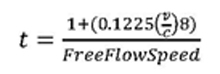
(Source: Speed Adjustments Using Volume-Delay Functions, TMIP Technical Synthesis, January 2009.)

where: t = travel rate (hours per mile)
v = hourly volume
c = capacity

4. Estimate incident delay for base and deployed cases using the relationships from the ITS Deployment Analysis System (IDAS); combine with recurring delay to get total delay and the overall travel time index (TTI) for each PeMS section.

Table 25. Operations deployment scenarios.

Strategy	Typical Option	Aggressive Option
Ramp Metering	+3 percent capacity	+5 percent capacity
Incident Management	-25 percent incident duration	-35 percent incident duration
Traveler Information: DMS	-0.5 percent total delay	Included in ATDM
Active Traffic and Demand Management (VSL, lane control, queue warning, junction control)	not applicable	-10 percent total delay

5. Fit a logistic function to the data to predict the mean TTI after deployment as a function of the mean TTI before deployment:

Figure 29. Equation. MeanTTI prime.

(Source: Cambridge Systematics, Inc.)

6. Develop predictive equations for the 50^th and 80^th percentile TTI as a function of the mean TTI by fitting sigmoidal functions to the PeMS data for I-580 and I-880 separately. For example:

Figure 30. Equation. MeanTTI superscript 80.

(Source: Cambridge Systematics, Inc.)

7. Factor the empirical TTI percentiles (from the PeMS data) by the ratio of the deployed TTI to the base TTI.

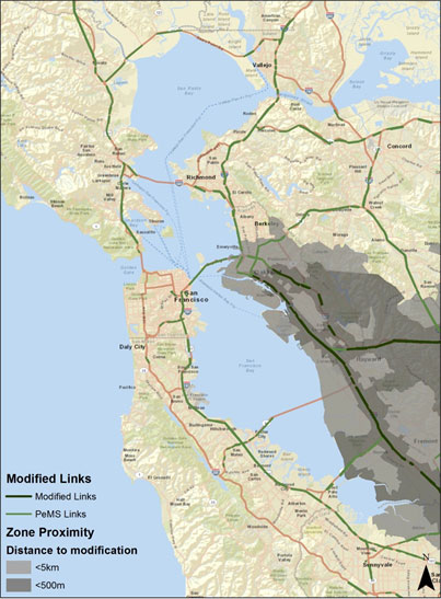
The links of I-880 and I-580 selected for the sensitivity testing are depicted in Figure 31, along with the distance from these links that are used to tabulate the simulation results below.

Figure 31. Map. Links modified for scenarios.

(Source: Cambridge Systematics, Inc.)

Sensitivity Analysis Results

Having constructed two scenarios, we then test these scenarios on the entire nine-county San Francisco Bay Area, using an adapted version of UrbanSim for this purpose (Waddell, 2002; Waddell, 2011). The design for the sensitivity tests was intended to help isolate the impacts of two levels of modifications to the 80^th percentile travel times on selected links on I-880 and I-580 in order to bring those times closer to the median values, a change that would reflect a reliability improvement with no change in median travel time. Note that this would underestimate the expected effects of operational improvements, since it avoids reflecting the impact on median travel times. But for our research objectives, this design was preferred in order to more directly assess the reliability impacts in the aggregate.

We structured the simulation to run over six iterations, though we constrained the control totals to be static, and the real estate supply to be static, in order to focus on real estate prices and demand effects. We assumed constant and low relocation rates for firms and households, with differential rates for renters and owners. Given our sensitivity testing design, we focus on the real estate effects on prices and rents, as the location choice changes are extremely small. In further extensions of this work, we may explore real estate supply and location choice impacts in more depth.

Sensitivity tests were run on three alternatives, one of which is the reference or base case. In the reference case we leave the travel times as observed in the PeMS data for all links in the network. In Scenarios 1 and 2, we modify the selected I-880 and I-580 links as shown in Table 26. In Table 26, we provide a summary of the simulation results of the two operations deployment scenarios compared to the baseline scenario in which no changes are made to travel times.

Table 26. Operations deployment scenario results compared to baseline.

Home Prices Scenario 1	$630.9	$594.9	$-41.7	$1,184.1
Home Prices Scenario 2	$1,392.7	$1,469.9	$-498.5	$2,364.1
Home Prices Scenario 1	1.0 percent	0.6 percent	0.0 percent	0.2 percent
Home Prices Scenario 2	2.2 percent	1.5 percent	-0.1 percent	0.3 percent
Residential Rent Scenario 1	$1.6	$1.2	$-0.3	$2.6
Residential Rent Scenario 2	$3.5	$3.3	$-1.7	$5.1
Residential Rent Scenario 1	0.5 percent	0.2 percent	0.0 percent	0.1 percent
Residential Rent Scenario 2	1.0 percent	0.6 percent	0.0 percent	0.1 percent
Nonresidential Rent Scenario 1	$14.0	$9.7	$99.2	$122.9
Nonresidential Rent Scenario 2	$31.4	$25.2	$245.1	$301.8
Nonresidential Rent Scenario 1	0.4 percent	0.2 percent	0.1 percent	0.1 percent
Nonresidential Rent Scenario 2	0.9 percent	0.6 percent	0.2 percent	0.2 percent
Prices and rents are in millions. Rents are annual.

The magnitudes of the impacts of the operations deployment scenarios are relatively modest in percentage terms, as would be expected for such an intervention. The largest percentage impacts occur on residential property values for owner-occupied units, with a 1.0 percent impact in the nearest homes in Scenario 1, and a 2.2 percent impact in Scenario 2. These effects decay significantly between 0.5 kilometers and 5 kilometers from the impacted highway segments, and are 0.1 percent or less beyond 5 kilometers. Interestingly, the effects remain positive when cumulated across the entire region, amounting to 0.2 percent of total owner-occupied property values in Scenario 1, and 0.3 percent in Scenario 2. When considered in absolute terms, the size of these impacts is impressive: the cumulative regional impact on owner-occupied property values is $1.184 Billion in Scenario 1, and $2.364 billion in Scenario 2. It would appear that reliability improvements are rather highly valued by homeowners, and there are many properties that would be affected by such changes, leading to very substantial regional impacts.

Results for residential rental properties also are impacted substantially by the operations deployment scenarios, though the percentage and absolute values of these impacts are smaller. The percentage impacts on annual rents were 0.5 percent in the closest properties in Scenario 1, and 1.0 percent in those properties in Scenario 2. Cumulative regional effects were 0.1 percent for both scenarios. The annual impact of the scenarios across the region was estimated to be $2.6 in Scenario 1, and $5.1 in Scenario 2. Note that these are annual rents, and have not been converted to price-equivalents for comparison to owner-occupied housing.

To give another frame of reference for these impacts, the owner-occupied homes within 0.5 kilometers of the affected highways are estimated to gain $2,600 on average in Scenario 1, and $5,800 in Scenario 2. Annual rents would increase by $212 in Scenario 1 and $454 in Scenario 2 on renter-occupied units, suggesting that there could be distributional impacts to consider from such improvements, with property owners reaping the windfall, and renters potentially bearing heavier rent burdens.

Nonresidential rents also were found to rise significantly as a consequence of these operations deployment scenarios. Space within 0.5 kilometers of the affected highway segments would be estimated to rise by $14.0 million (0.4 percent) in Scenario 1, and $31.5 million (0.9 percent) in Scenario 2. Across the region, these impacts accumulate to $122.9 million (0.1 percent) in Scenario 1, and $301.8 million (0.2 percent) in Scenario 2. These also are annual impacts, so the long-term impacts would accumulate across multiple years, with some discount rate.

Conclusions

This research has explored a question that has not received prior research attention. In light of the results of both our empirical research results, and the sensitivity tests of plausible operations deployment scenarios, we find that the reliability of accessibility does impact real estate markets significantly. It clearly impacts residential prices and rents, as well as nonresidential rents. The magnitude of these effects is highest close to the interventions, but extends well beyond the immediate area, and our results suggest that there may be substantial regional benefits to improving travel-time reliability that have been previously overlooked, resulting in an underestimate of the benefits from such projects.

There are of course caveats on our research findings. First, the sensitivity tests were constructed somewhat manually and in a way that lent itself to helping to answer our questions on the impact of reliability improvements while holding median travel times constant. In reality, operations improvements would generally improve both the median and the 80^th percentile travel times. Second, we only studied one metropolitan area, during one period of time. The San Francisco Bay Area may have idiosyncrasies that might make our results less general. We think the research should be replicated in other metropolitan areas that vary in size and other dimensions. Finally, we focused on roadway operations and travel-time reliability, and transit reliability was not part of the scope of this research. Given the magnitude of the impacts we found, we think it would be promising to conduct similar research on transit reliability.

One sobering aspect of this research is that it begins to suggest that the state of the practice, and to a large extent, even the state of the art in travel modeling, is designed to squeeze out information on travel time variability, rendering the models useless for examining the impacts of operations changes on reliability. Our initial hope was to be able to combine land use modeling and transport modeling in a way that consistently dealt with travel time distributions, but this was not possible with available travel models. It seems that much more research needs to be oriented in the direction of developing travel models that generate well-calibrated distributions of travel times, rather than a single, fixed-point result of an assumed equilibration process. It turns out that reliability is more important than had been previously assumed, and both travel and land use models should reconsider how best to incorporate travel time variability into their design.

References

Note: Due to the large number of references for this chapter, we have organized them as endnotes rather than footnotes.

Alonso, W. (1960). A theory of the urban land market, Papers in Regional Science 16(1): 149-157.

Bates, J., Polak, J., Jones, P. and Cook, A. (2001). The valuation of reliability for personal travel, Transportation Research Part E: Logistics and Transportation Review 37(23): pp. 191-229.

Ben-Akiva, M. and Lerman, S. R. (1987). Discrete Choice Analysis: Theory and Application to Travel Demand, The MIT Press, Cambridge, Massachusetts.

Brownstone, D. and Small, K. A. (2005). Valuing time and reliability: assessing the evidence from road pricing demonstrations, Transportation Research Part A: Policy and Practice 39(4): 279-293.

Clark, W. A. V. and Lierop, W. F. J. V. (1986). Residential mobility and household location modeling, Handbook of Regional and Urban Economics, Volume 1, Elsevier Science Publishers BV, pp. 97-132.

DiPasquale, D. and Wheaton, W. (1996). Urban Economics and Real Estate Markets, Prentice Hall: Englewood Cliffs, New Jersey.

Downs, A. (2004). Still Stuck in Traffic: Coping with Peak-Hour Congestion, The Brookings Institution, Washington, D.C.

Edmonds, Radcliffe G., J. (1983). Travel time valuation through hedonic regression, Southern Economic Journal 50(1): pp. 83-98.

Ettema, D., Tamminga, G., Timmermans, H. and Arentze, T. (2005). A microsimulation model system of departure time using a perception updating model under travel time uncertainty, Transportation Research Part A 39: 325-344.

Fosgerau, M. and Karlström, A. (2010). The value of reliability, Transportation Research Part B: Methodological 44(1): 38-49.

Giuliano, G. (2004). The Geography of Urban Transportation, 3^rd edn, Guilford Publications, Incorporated, chapter Land Use Impacts of Transportation Investments – Highway and Transit, pp. 237-273.

Gordon, P. and Richardson, H. (1997). Are compact cities a desirable goal?, Journal of the American Planning Association 63(1): 95-106.

Greene, W. H. (2002). Econometric Analysis, 5^th edn, Pearson Education. Hansen, W. (1959). How accessibility shapes land use, Journal of the American Institute of Planners 25(2): 73-76.

Hoch, I. and Waddell, P. (1993). Apartment rents: Another challenge to the monocentric model, Geographical Analysis 25(1): 20-34.

Lam, T. C. and Small, K. A. (2001). The value of time and reliability: measurement from a value pricing experiment, Transportation Research Part E: Logistics and Transportation Review 37(23): 231- 251.

Lee, B., Waddell, P., Wang, L. and Pendyala, R. (2010). Reexamining the influence of work and nonwork accessibility on residential location choices with a microanalytic framework, Environment and planning. A 42(4): 913.

Lerman, S. (1977). Location, housing, automobile ownership, and the mode to work: A joint choice model, Transportation Research Board Record 610: 6-11.

Li, Z., Hensher, D. A. and Rose, J. M. (2010). Willingness to pay for travel-time reliability in passenger transport: A review and some new empirical evidence, Transportation Research Part E: Logistics and Transportation Review 46(3): 384-403.

Lomax, T., Schrank, D., Turner, S. and Margiotta, R. (2003). Selecting travel reliability measures, Technical report, Texas Transportation Institute.

McFadden, D. (1974). Conditional logit analysis of qualitative choice behavior, in P. Zarembka (ed.), Frontiers in Econometrics, Academic Press, New York, pp. 105-142.

McFadden, D. (1978). Modeling the choice of residential location, in A. Karlqvist, L. Lundqvist, F. Snickars and J. Wiebull (eds), Spatial Interaction Theory and Planning Models, North Holland, Amsterdam, pp. 75-96.

McFadden, D. (1981). Econometric models of probabilistic choice, in C. Manski and D. McFadden (eds), Structural Analysis of Discrete Data with Econometric Applications, MIT Press, Cambridge, Massachusetts, pp. 198-272.

Mills, E. (1992). Office rent determinants in the Chicago area, Real Estate Economics 20(2): 273-287.

Muth, R. F. (1961). The spatial structure of the housing market, Papers in Regional Science 7(1): 207-220.

Nam, D., Park, D. and Khamkongkhun, A. (2005). Estimation of value of travel-time reliability, Journal of Advanced Transportation 39(1): 39-61.

Nelson, J. P. (1977). Accessibility and the value of time in commuting, Southern Economic Journal 43(3): pp. 1321-1329.

Noland, R. B. (2001). Relationships between highway capacity and induced vehicle travel, Transportation Research Part A: Policy and Practice 35(1): 47-72.

Pendyala, R., Konduri, K., Chiu, Y., Hickman, M., Noh, H., Waddell, P., Wang, L., You, D. and Gardner, B. (2012). An integrated land use-transport model system with dynamic time-dependent activity-travel microsimulation, 91^st Annual Meeting of the Transportation Research Board, Washington, D.C.

Quigley, J. (1976). Housing demand in the short-run: An analysis of polytomous choice, Explorations in Economic Research 3: 76-102.

Rosen, K. (1984). Toward a model of the office building sector, Real Estate Economics 12(3): 261-269.

Rosen, S. (1974). Hedonic prices and implicit markets: Product differentiation in pure competition, Journal of Political Economy 82(1): 34-null.

Shukla, V. and Waddell, P. (1991). Firm location and land use in discrete urban space: A study of the spatial structure of Dallas-Fort Worth, Regional Science and Urban Economics 21(2): 225- 253.

Small, K. A., Winston, C. and Yan, J. (2005). Uncovering the distribution of motorists’ preferences for travel time and reliability, Econometrica 73(4): 1367-1382.

Train, K. E. (2003). Discrete Choice Methods with Simulation, Cambridge University Press.

Train, K. E. (2009). Discrete Choice Methods with Simulation, Cambridge University Press.

van Lint, J., van Zuylen, H. J. and Tu, H. (2008). Travel time unreliability on freeways: Why measures based on variance tell only half the story, Transportation Research Part A 42: 258-277.

Waddell, P. (1997). Household Choice and Urban Structure: A Re-Assessment of the Behavioral Foundations of Urban Models of Housing, Labor and Transportation Markets, Ashgate, University of Texas at Dallas.

Waddell, P. (2000). A behavioral simulation model for metropolitan policy analysis and planning: Residential location and housing market components of UrbanSim, Environment and Planning B: Planning and Design 2000 27(2): 247-263.

Waddell, P. (2002). UrbanSim: Modeling urban development for land use, transportation, and environmental planning, Journal of the American Planning Association 68(3): 297-314.

Waddell, P. (2007). Accessibility and residential location: the interaction of workplace, housing tenure, residential mobility and location choice, in J. Preston, F. Pagliara and D. Simmonds (eds), Modeling Residential Location Choice, Ashgate. in press.

Waddell, P. (2011). Integrated land use and transportation planning and modeling: Addressing challenges in research and practice, Transport Reviews 31(2): 209-229.

Waddell, P., Berry, B. J. and Hoch, I. (1993). Residential property values in a multimodal urban area: New evidence on the implicit price of location, Journal of Real Estate Finance and Economics 7: 117-141.

Waddell, P. and Nourzad, F. (2002). Incorporating non-motorized mode and neighborhood accessibility in an integrated land use and transportation model system, Transportation Research Record (1805): 119-127.

Waddell, P. and Shukla, V. (1993). Employment dynamics, spatial restructuring, and the business cycle, Geographical Analysis 25(1): 35-52.

Waddell, P. and Shukld, V. (1993). Manufacturing location in a polycentric urban area: a study in the composition and attractiveness of employment subcenters, Urban Geography 14(3): 277-296.

Waddell, P. and Ulfarsson, G. F. (2003). Accessibility and agglomeration: Discrete-choice models of employment location by industry sector, 2003 Annual Meeting of the Transportation Research Board, Washington, D.C.

Waddell, P., Ulfarsson, G., Franklin, J. and Lobb, J. (2007). Incorporating land use in metropolitan transportation planning, Transportation Research Part A: Policy and Practice 41: 382-410.

Waddell, P., Wang, L., Charlton, B. and Olsen, A. (2010). Microsimulating parcel-level land use and activity-based travel: Development of a prototype application in San Francisco, Journal of Transportation and Land Use 3(2): 65-84.

Wang, L., Waddell, P. and Outwater, M. (2011). Incremental integration of land use and activity-based travel modeling: Work-at-home and out-of-home workplace choices. Transportation Research Board 89^th Annual Meeting Compendium of Papers DVD.

You may need the Adobe® Reader® to view the PDFs on this page.