Travel and Emissions Impacts of Highway Operations Strategies

Chapter 2. Current Knowledge Base

Introduction

A literature review was conducted for the study. Additionally, three topics were treated in-depth and developed as separate white papers:

• The operations versus new capacity impacts of changes in travel-time reliability, average travel time, and monetary travel cost on travel behavior.
• Implications of induced demand for estimating impacts and social⁄user benefits (acknowledging geographic and temporal considerations).
• The effect of accessibility and reliability on land use patterns.

Each of these efforts is summarized in this chapter.

Literature Review

Assessing the Impacts of Operations Strategies

Evaluation of Models Used in Analysis of Operations Strategies

Planning and simulation models that have been used for decades to evaluate projects impacts, including air quality, have not accounted for nonrecurring events and congestion. Models generally use data for an average day or average peak or off-peak time period during the day. Since these models are often calibrated against daily traffic volumes they do account for nonrecurring congestion to some extent, but do not fully capture the impacts of incidents, work zones, adverse weather, and special events on performance measures such as travel time, crash rates, fuel consumption, and air quality.

Several recent and well-documented trends in transportation have led to greater interest in modeling nonrecurring congestion and its impacts on system performance:

• For a number of reasons, major increases in roadway capacity are not likely any time in the foreseeable future. Available funds are limited and must be used to primarily to maintain and⁄or rebuild the existing infrastructure. New capacity is extremely expensive due to the proximity of development and environmental constraints. As a result, transportation agencies are focusing more on operational strategies that are designed to optimize the capacity of the existing system.
• More transportation agencies, particularly State DOTs, are managing based on specific performance measures. There is interest in quantifying these measures wherever possible. Agencies are under increasing pressure to justify funding requests by demonstrating that they are making most efficient use of the dollars being provided. Agencies also are more conscious of the need to communicate their activities to the public. “Dashboard” reports, that show high-level metrics easily understood by laypersons are becoming more popular with State DOTs and other transportation agencies. These reports increasingly include measures that address agency effort to reduce the impacts of nonrecurring congestion.
• The availability and quality of detailed data that can be used to measure system performance continue to increase. ITS and Transportation Management Centers have continued to expand and mature. These systems are not only monitoring more highways in real time but are producing archives of data on system volumes and speeds that are largely untapped for their research potential. In the past few years, private companies have begun to collect and compile probe data from various sources such as commercial fleets and cell phones. They are selling this information to public agencies, enabling them to monitor speeds on much greater proportions of their highway systems. These data sources allow coverage of rural interstates and major arterials that would not be financially realistic if investment in ITS and communications infrastructure were required. Connected vehicle technology, which is now in its infancy as a planning and research tool, provides much greater potential to monitor movements across the entire system through collection and processing of anonymous data from large numbers of individual vehicles.
• Through the SHRP 2 program and other research efforts, the transportation community is gaining a much better understanding of the impact of nonrecurring events and the concept of reliability. Annual results from the Texas Transportation Institute’s annual Urban Mobility Report receive wide attention in the media and used by the public to understand changes in congestion levels. Concepts such travel-time index and buffer index are starting to be used by private and public traffic information services to explain delays to the public and allow changes to be measured. There are many research efforts ongoing to better understand the components and causes of nonrecurring congestion and its impacts.

Measurement of nonrecurring congestion is a focus of much of the research summarized in this chapter. The goal of many of these research efforts is to enable practitioners to predict the impacts of nonrecurring events in real time and communicate that information to the public. A next step would be to provide guidance on whether to use alternative routes and which routes to use. It can also enable system operators to implement mitigating strategies such as dynamic routing of emergency vehicles to incident scenes, retiming of signals or ramp meter rates on alternative routes and implementation of variable speed limits. As data resources and archives are developed over time they can be used to refine these strategies.

Systemwide Congestion and Reliability Analysis

One of the major findings under this category is the increasing use of real-time traffic data by researchers to understand congestion, reliability, and operational strategies. Hainen, Wasson, et al. proposed a technique for assessing route choice and travel time using an anonymous Bluetooth MAC address sampling technique as a surrogate for license plate matching to assess route choice. The authors of this paper concluded that the Bluetooth sampling technique is very cost-effective to deploy and although the results are approximate, the direct measurement of travel times and route choice is potentially very useful for public agencies assessing mobility and travel-time reliability along alternative routes, particularly distribution of traffic between different alternate routes (Hainen, Wasson, et al., Purdue University, “Estimating Route Choice and Travel-time reliability Using Field Observations of Bluetooth Probe Vehicles,” TRB 2011 Annual Meeting, 11-0462). The benefits of this technique have great potential for better understanding of diversion strategies and could help operators to refine and these strategies make them more effective. Measurement of speeds and travel time using multiple sources of data also was the subject of tried on urban streets in London. The documented technique also has application in performance measurement of freeway management and traveler information strategies (Hasan, Choudhury, Ben-Akiva, Emmonds, “Modeling Travel Time Variations on Urban Links in London,” TRB 2011 Annual Meeting, 11-0473). Enhancements to Dynamic Traffic Assignment models for evaluation of operational improvements were reviewed by Kittelson, et al. (Kittelson, Rouphail, Williams and Zhou, “Analyzing Operational Improvements as an Alternative to Traditional Highway Construction,” TRB Annual Meeting, 11-0714). Model improvements tested included stochastic capacity for freeway and arterials, improved representation of arterial bottlenecks, and use of the findings to represent day-to-day learning capability.

Another effort to model the impacts of ATIS on system performance was developed by Li, Zhou, et al. (Li, Zhou, Rouphael, “Planning Level Methodology for Evaluating Traveler Information Provision Strategies under Stochastic Capacity Conditions) who modeled two categories of ATIS users using stochastic capacity, travelers with perfect real-time information, and travelers with some knowledge based on historical patterns.

Another advanced technique identified was the multicriterion dynamic user equilibrium (MDUE) traffic assignment model that incorporates travel-time reliability in addition to them more traditional variables of travel time and out-of-pocket cost in the assignment process. The model was tested to look at road pricing schemes in the New York metropolitan region (Jiang and Mahmassani, “Congestion Pricing, Heterogenous Users and Travel-time reliability: Multi-Criterion Dynamic User Equilibrium Model and Efficient Implementation for Large Scale Networks”). Another research effort involved development and testing of a stochastic network simulation model that can generate random flow breakdowns at different levels, capture the traffic characteristics at the beginning of the breakdown and evaluate travel time variability (Jing and Mahmassani, “Predicting Flow Breakdown Probability and Duration in Stochastic Network Models: Impact on Travel-time Reliability”).

Incident Management

Several studies were identified that tested analytical techniques for estimating the duration and traffic flow impacts of incidents. The ability to do this is important in making informed operational decisions, including:

• Stationing and response routes for service vehicles.
• Implementation of lane closures and⁄or detours.
• Traveler information messages.
• Allocation of resources to incident management.

With greater geographic coverage through CCTV and larger volumes of traffic and speed data coming back to TMCs, analytical tools are needed to take advantage of these opportunities. One of the reports documents the use of the I‑MIT model (Khattak, Wang and Zhang, “I‑MIT: A Tool for Dynamically Predicting Incident Durations, Secondary Incident Occurrence, and Incident Delays). Roadway inventory, traffic, and incident data from the Hampton Roads (Virgina) Traffic Operations Center were used to dynamically predict incident durations, secondary incident occurrence, and associated delays.

Resources – Manuals Guidebooks and Databases

The literature search identified a number of resources that practitioners can use today that document analytical tools, methods, and data for analysis of travel time and reliability. A current major initiative is the Benefit⁄Cost Desk Reference for Management and Operations that will be issued by FHWA later this year. This reference guide will document techniques for conducting benefit⁄cost analysis for ITS and operational improvements. Other key references include documentation of the FHWA’s Traffic Analysis Tools Program, the U.S. DOT Integrated Corridor Management Program, and a Guidebook on the Congestion Management Process. Tools specific to ITS analysis also are included such as the ITS Deployment Analysis System (IDAS), the Highway Economic Requirements System (HERS) and the Screening for ITS Spreadsheet (SCRITS). There are several manuals designed to help State and MPO planners incorporate ITS, operational, and safety issues into their planning processes.

Emissions Models for Testing Operations Strategies

The following modal emission models were selected for inclusion in the project. A short description of each one and the reason for their selection is provided below. Table 3 presents a summary analysis for modal emission models.

Table 3. Comparison of modal emissions models.

	Modal Emissions Model MOVES	Modal Emissions Model CMEM (NCHRP 25‑11)	Modal Emissions Model MEASURE	Modal Emissions Model CDOH Method	Modal Emissions Model CALINE 4	Modal Emissions Model VT-Micro	Modal Emissions Model TRAQSIM (UCF)	Modal Emissions Model HYROAD NCHRP 25‑6)	Modal Emissions Model NCHRP 25‑14
Pollutant CO	included	included	included	included	included	included	included	included	included
Pollutant NOx	included	included	included	included	NO2	included			included
Pollutant VOC	included	HC	included	HC		HC			HC
Pollutant PM10	included				included				included
Pollutant PM2.5	included				included				included
Pollutant GHG	included	CO2				CO2
Pollutant Fuel Usage	Energy Consumption					included
Current Status – Up to date and supported	Yes.	Yes.	No.	No.	Yes.				No.
Input – Modal activity inputs	Operating Mode Distributions or Vehicle Trajectories.	Second-by-second vehicle speed, acceleration, road-grade, accessory usage (e.g., A⁄C).			Cruise speed, acceleration time, deceleration time, maximum idle time, minimum idle time.	Second-by-second speed and acceleration.	Second-by-second speed and acceleration.
Input – Load producing effects included (road-grade, A⁄C use, etc.)	Yes.	Yes.				No.
Input – Details on emissions calculation methods	Lookup table of VSP and average-speed bins.	Engine-power demand model.		Modal multipliers convert average-speed emissions factors.	Modal multipliers convert average-speed emissions factors.	Fuel consumption and emission rates predicted directly from empirical models.	Modal multipliers convert average-speed emissions factors.
Input – Considers vehicle operating history	No (converts vehicle trajectories to operating mode distribution).	Yes, for batch and GUI mode. Not for table mode.
Input – Strength	General.	General.	GIS applications.	Simple.	Intersection dispersion modeling based on modal emissions factors.		Updated version of CDOH and CALINE models, simpler than CMEM.	CO emissions at intersections.	Heavy-duty for NOx and HC (does not do CO or PM well). Results used for speed correction factors in other emission rate models.

• MOVES – The Motor Vehicle Emissions Simulator (MOVES) is now the EPA’s official model for estimating emissions from highway vehicles. It covers all pollutants desired and, when used in project mode, it accepts modal activity inputs. It became available for official SIP and conformity work in January 2010 and is fully supported by the EPA.
• CMEM – The Comprehensive Modal Emissions Model (CMEM) was developed by UC Riverside as part of NCHRP Project 25-11. It models emissions by estimating physical properties of engine-power demand using second-by-second data on vehicle speed, acceleration, road-grade, and accessory usage. Therefore, it requires a large amount of data to run, but can be integrated into microsimulation models, such as Paramics, to automate the transfer of this data without intermediate input and output files. It covers all pollutants except for particulate matter.
• VT-Micro – Developed by Virginia Tech, VT-Micro predict fuel consumption and emission rates based on empirical models. It covers all pollutants except for particulate matter and has been incorporated into the INTEGRATION microsimulation model.

The following modal emission models were excluded from further consideration. A short description of each one and the reason for their exclusion is provided below.

• MEASURE – The Mobile Emissions Assessment System for Urban and Regional Evaluation (MEASURE) was developed by Georgia Tech under a cooperative agreement with the EPA and FHWA. The model contributed to the body of knowledge for modal emissions modeling, but it was folded into the MOVES creation effort and is no longer up to date or supported. It also does not have a greenhouse gas or fuel usage component.
• CDOH Method – The Colorado Department of Highways (CDOH) created this method in the early 1980s to develop emission factors that were representative of modal activities. This relatively simple method creates modal multipliers to convert average-speed emission factors to emission factors for each modal activity (accelerations, decelerations, cruise, etc.). This method does not include greenhouse gases or fuel usage and appears to no longer be used as the Colorado DOT recommends using the MOVES model for project-level hot-spot analysis.
• CALINE4 – The California Department of Transportation’s California Line Source Dispersion Model (CALINE) is mainly for predicting pollutant concentrations for project-level analysis. However, for intersections it contains a method to convert average-speed emission factors to modal emission factors, similar to the CDOH method. It does not include greenhouse gas emissions or fuel usage and is only for light-duty vehicles at intersections.
• TRAQSIM – The Transportation Air Quality Simulation Model (TRAQSIM) was developed by the University of Central Florida (UCF) as an updated version of the modal multiplier methods employed by CDOH and CALINE as described above. It is based on more recent vehicle testing conducted in the 1990s. While its simplicity is an advantage it appears to only model carbon monoxide (CO).
• HYROAD – The Hybrid Roadway Model (HYROAD) was created under NCHRP 25-6 to integrate a traffic simulation model, emissions model, and a dispersion model into one. However, this model is only for intersections and only covers carbon monoxide (CO) and particulate matter (PM).
• NCHRP 25-14 Method – This method of estimating emissions from heavy trucks using second-by-second speed and acceleration data was deemed to provide valid results only for NO_x and HC, but did not provide valid results for CO or PM. The most important results from this study were the identification of the need to update speed correction factors in the MOBILE model for NO_x and HC.

Demand Effects of Transportation Improvements

A summary of the separate literature review that was prepared and how it is useful for the current study is provided below.

• It is extremely important to separate the short- and long-run components of induced travel. It also is critical to identify the independent variable: studies have related induced demand to changes in travel time, lane-miles (a surrogate for roadway capacity), and total travel costs. For operations strategies, the most desirable independent variable is travel time, and the more recent studies use travel time as the independent variable. (However, most studies in the literature use lane-miles.) An advanced modeling framework that incorporates an activity-based model (ABM) uses interzonal travel times to allocate travel activities.
• Short-run elasticities (e.g., diversion of existing trips) have been found to be smaller than long-run elasticities. While additional traffic generated in the short run is appropriate for facility planning, researchers have generally held that, except for modal diversion, long-run changes are more appropriately tagged as induced demand, i.e., new or longer trips that would not have been made without the improvement.
• A variety of analysis strategies have been used to develop induced demand elasticities, and all of the studies suffer from the inability to control various exogenous factors. The most common types of analyses are:
  • Cross-sectional analysis of travel surveys.
  • Facility-specific time series analysis.
  • Macroscopic time series (e.g., relating total VMT to total lane-mile growth).
• Because of the influence of exogenous factors, it is likely that the induced demand effect has been overstated in older studies (see Table 3). A good example is when Cohen reexamined his previous work with additional controls and found that his original elasticities were larger.
• One of the major exogenous factors that is difficult to control is expected growth. Urban transportation improvements (capacity expansion, demand management, and operations) are almost universally made where severe congestion exists, growth is expected to be high, or both. Therefore, depending on the analysis method, at least some of the observed demand growth is incorrectly assigned as “induced” – analysts expected there to be growth. Cross-sectional survey analysis does not suffer from this problem (it has others) but most time series (i.e., longitudinal) analyses do.
• With respect to induced demand as a function of lane-miles, an important distinction not controlled for in macroscopic time series analyses is expansion of existing facilities (e.g., additional lanes) as opposed to totally new capacity (e.g., a new highway or rail line). New capacity will dramatically shift development patterns and create economic opportunities where none previously existed. The effect will be smaller with capacity expansion of existing facilities.
• With regard to operational strategies and demand shifts, most operations strategies are targeted on congestion during peak periods, with the exception of incident management and even there the primary effect will be during peak periods. For example, ramp metering, lane control, and speed harmonization only provide benefits during congested times. The amount of discretionary travel during the peaks is limited, as most of the trips are work-based, especially during the morning peak. (Existing travelers cannot make additional work trips.) Although it is not explicitly stated in the studies reviewed, we do not believe that they are based on peak travel, but rather total travel during the day, when more discretionary trips are present. We postulate that peak travel – the focus of operations – is more inelastic than travel made outside of the peak.
• The long-run elasticity used in the Highway Economic Requirements System (HERS) model (-1.0), is on the high side of the two other studies reviewed where travel time was the independent variable. Further, there is a concern about how elasticities that are developed at the trip level should be applied to a facility-based improvement. This argument says that it is the percent change in travel time for the entire trip – not just that part of the trip on the improved facility – that should be used. Note that this is not an issue for the modeling frameworks with an ABM component as total trip (interzonal) travel times are computed and used.
• One study by work by Toole-Holt et al.demonstrated that in the U.S., the average daily travel time per person increased by 1.9 minutes per year between 1983 and 2001, and that the majority of this increase came from increased trip-making by travelers. There are two major implications of this finding:
  • Time series studies of induced demand, especially for this period of time, ignore this effect, which is substantial.
  • Increased trip-making occurred even as urban delay quadrupled during this period, suggesting that the induced demand effect is a minimal player in comparison to other exogenous travel factors.

Short-term elasticities of demand with travel time or capacity are routinely observed and included in the traditional travel demand forecasting methods used by transportation planners; it is the long-run effect that is more difficult to ascertain. Nearly all past studies on induced demand have concluded that a long-run induced demand effect exists, yet there is ample evidence that the effect is smaller than previously indicated. Further, operations strategies are targeted at congestion and it is unlikely that they would induce additional discretionary trips outside of peak periods. For example, improving a signalized highway to full access control would provide lower travel times to travels in both peak and nonpeak periods.

Given the problems with past studies, use of an advanced modeling framework will provide insight into the issue of induced demand and operations. Table 4 shows the various components of induced demand (as identified in SHRP 2 Project C04) (Parsons Brinckerhoff et al., “Improving Our Understanding of How Highway Congestion and Pricing Affect Travel Demand,” SHRP 2 Project C04, Transportation Research Board, 2013) and that with the exception of residential location and land use effects, all of the induced demand components can be modeled.

Table 4. Ability of activity-based modeling frameworks to accommodate demand shifts.

Choice Dimension	Time Scale for Modeling	Expected Impact	Ability to Model
Network Route Choice	Short term – Trip episode	Stratified response by user group.	Modeled in traffic assignment
Preroute Choice (Toll versus Nontoll)	Short term – Trip episode	Stratified response by user group.	Modeled in ABM portion
Car Occupancy	Short term – Tour⁄trip episode	Planned and casual carpool.	Modeled in ABM portion
Mode Choice	Short term – Tour⁄trip episode	Shift to transit, especially to rail and for low/medium-income groups.	Usually modeled in ABM portion
Time of Day⁄Schedule	Short term – Tour⁄trip episode	Peak spreading.	Modeled in ABM portion
Destination/Stop Location	Short term – Tour⁄trip episode	Improved accessibility effect combined with negative pricing effect on trip distribution for nonwork trips.	Modeled in ABM portion
Joint Travel Arrangements	Short term – Within day	Planned carpool/escorting.	Modeled in ABM portion
Tour Frequency, Sequence, and Formation of Trip Chains	Short term – Within day	Lower tour frequency and higher chaining propensity.	Modeled in ABM portion
Daily Pattern Type	Short term – Weekly (day-to-day)	More compressed workdays and work from home.	Modeled in ABM portion
Usual Locations and Schedule for Nonmandatory Activities	Medium term – One month	Compressed⁄chain patterns; weekly planned shopping in major outlets.	Modeled in ABM portion
Household⁄Person Mobility Attributes (Transponder, Transit Path, Parking Arrangements at Work)	Medium term – One to six months	Higher percentage of transponder users and parking arrangements for high incomes, higher percentage of transit path holders for low incomes.	Not modeled; likely to have a very small effect
Household Car Ownership Choice	Long term – One year	Stratified response by income group: Higher car ownership for high incomes; Lower car ownership for low incomes.	Usually modeled in ABM portion
School⁄University Location and Schedule	Long term – One to five years	Choice by transit accessibility; flexible schedules.	Sometimes modeled in ABM portion
Job⁄Usual Workplace Location and Schedule	Long term – One to five years	Local jobs for low incomes; compressed/flexible schedules.	Sometimes modeled in ABM portion
Residential Location	Long term – More than five years	Income stratification: High-income suburbs around tolls roads; Low-income clusters around transit.	Need land use model integrated with travel model
Land Use Development	Long term – More than five years	Urban sprawl if no transit; otherwise shift to transit.	Need land use model integrated with travel model

The Impact of Capacity and Operations Improvements on Travel Time, Travel-time Reliability, and Traveler Behavior

This investigation focused on travel time and travel-time reliability (henceforth, just “reliability”) from two perspectives:

1. How do capacity and operations strategies affect travel time and reliability? What is the mechanism for their effect and what is the scale⁄magnitude of the effect?
2. How do changes in travel time and reliability affect the behavior of travelers in terms of trip choices? How can these choices be modeled?

Definition of Travel-Time Reliability

Many definitions of reliability have been developed over the years. Most recently, the reliability definitions used by SHRP 2 projects all use the variability in travel times as the fundamental concept behind defining reliability. The common themes in the SHRP 2 definitions can be rolled into the following overarching definition.

Travel-time reliability is the variability in travel times that occur on a facility or a trip over the course of time, and is due to the interaction of the factors that influence travel times: fluctuations in demand, traffic control devices, traffic incidents, inclement weather, work zones, and physical capacity (based on prevailing geometrics and traffic patterns). The reliability of a facility or trip can be reported for different time slices, e.g., weekday-peak hour, weekday-peak period, and weekend.

A corollary to the basic definition of reliability as variability is the concept of failure, or its opposite, on-time (success). The underlying variability in travel times implies that a certain number of trips will be within an acceptable threshold, and thus will have “failed” or “succeeded.”

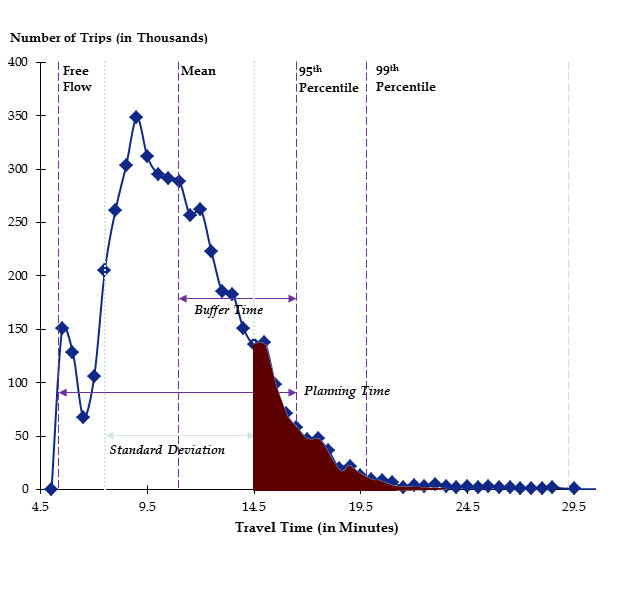
From a measurement perspective, reliability is defined from the distribution of travel times, for a given facility⁄trip and time slice, that occurs over a significant span of time; one year is generally long enough to capture nearly all off the variability caused by disruptions. A variety of different metrics can be computed once the travel time distribution has been established, including standard statistical measures (e.g., standard deviation, kurtosis), percentile-based measures (e.g., 95^th percentile travel time, Buffer Index), on-time measures (e.g., percent of trips completed within a travel time threshold, and failure measures (e.g., percent of trips that exceed a travel time threshold); see Figure 5.

The basic definition of travel-time reliability (variability in travel times) can be extended to include the notion of predictability, that is, the probability that a travel time for a facility or trip is within acceptable limits for the traveler, given that travel times are affected by interaction of demand fluctuations, traffic control devices, traffic incidents, inclement weather, work zones, and physical capacity. It can also be used to compare current conditions to history: is the travel time today “typical” of what happens or is it better than usual or near-worst case. However, both of these corollaries are based on establishing the variability over time, as defined by the travel time distribution.

In a broader sense, reliability is a dimension or attribute of congestion. Traditionally, the dimensions of congestion have been spatial (how much of the system is congested?), temporal (how long does congestion last?), and severity-related (how much delay is there or how low are travel speeds?). Reliability adds a fourth dimension: how does congestion change from day-to-day?

Relationship Between Travel Time and Reliability

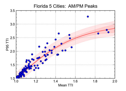
The notion that reliability can be thought of as an attribute of total congestion was verified empirically in SHRP 2 Project L03 and has been observed on a limited basis prior to that (Jones, E.G. (1988), Characterizing Travel Time Variability in a Commuting Corridor. Masters Thesis, Department of Civil Engineering, University of Texas at Austin. Also, more recently in: Improving Reliability on Surface Transport Networks, OECD, ISBN 978-92-82-10242-8, 2010). The basic relationship shown in Figure 6 was found to exist for multiple urban areas, multiple measures of reliability (the 95^th percentile travel time index is shown, but standard deviation and percent on time trips also exhibit a strong correlation), and for both individual links and travel time over an extended segment. What this means is that an estimate of the mean level of congestion is known, reliability metrics can be predicted. Project L03 developed a set of predictive equations for doing this; one example is:

Figure 4. Equation. 95^th percentile.

(Source: Cambridge Systematics et al., Analytic Procedures for Determining the Impacts of Reliability Mitigation Strategies, SHRP 2 Project L03, Transportation Research Board, 2013.)

Where: TTI is the travel time index.

Figure 5. Graph. The travel time distribution is the basis for defining reliability metrics.

(Source: Kittelson Associates et al., Incorporation of Travel-time reliability into the Highway Capacity Manual, Transportation Research Board, 2014.)

Figure 6. Scatter graph. Correlation between 95^th percentile TTI and mean TTI.

(Source: Cambridge Systematics, Inc.)

Mechanisms for Affecting Travel Time and Reliability

There are three basic mechanisms for changing both travel time and reliability:

1. Demand – can be reduced overall or shifted to less traveled routes and/or times of travel.
2. Capacity – additional highway space can be added or traffic control systems can be improved to provide an “effective” increase in capacity.
3. Disruptions – can decrease capacity and negatively influence traffic flow. These include:
   1. Incidents – lane and shoulder blockages drop the effective capacity significantly. “Rubbernecking” affects driver behavior and also impacts capacity.
   2. Work Zones – lane/shoulder closures and lane shifts drop the effective capacity significantly.
   3. Weather – affects driver behavior, sometimes drastically, leading to a drop in effective capacity.

Effect of Travel Time and Reliability on Traveler Behavior

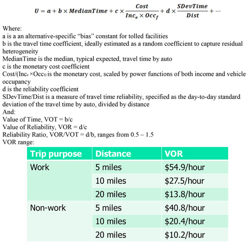
The concept of “extra impedance due to unreliable travel” is probably the best way to incorporate reliability into the modeling structure as an input. SHRP 2 Project C04, Improving Our Under standing of How Highway Congestion and Pricing Affect Travel Demand, used this approach where the impedance on a link can be captured as a generalized cost function that includes both the average travel time and its standard deviation (which is used as the indictor of reliability; Figure 7).

Figure 7. Equation. SHRP 2 Project C04’s generalized highway utility function.

(Source: PB Americas et al., Improving Our Understanding of How Highway Congestion and Pricing Affect Travel Demand, SHRP 2 Project C04, Transportation research Board, 2013.)

An alternative but conceptually similar approach can be based on the recent work of Small, Winston, and Yan (Small, K.A., C. Winston, and J. Yan. (2005) Uncovering the Distribution of Motorists’ Preferences for Travel Time and Reliability, Econometrica, 73(4), 1367-1382). They adopted the quantitative measure of variability as the upper tail of the distribution of travel times, specifically, the difference between the 80^th and 50^th percentile travel times. The authors argue that this measure is better than a symmetric standard deviation, since in most situations, being “late” is more crucial than being “early,” and many regular travelers will tend to build a “safety margin” into their departure times that will leave them an acceptably small chance of arriving late (i.e., planning for the 80^th percentile travel time would mean arriving late for only 20 percent of the trips).

Based on this work, the notion of “travel time equivalents” can be used, where reliability is equilibrated to average travel time. The calculation of travel time equivalents can then be constructed as:

Figure 8. Equation. TTE.

(Source: Dowling, Richard and Margiotta, Richard, Guide for Highway Capacity and Operations Analysis of Active Transportation and Demand Management Strategies, prepared for FHWA Office of Operations, June 2013.)

Where:

TTE is the travel time equivalent on the link.
MTT is the mean travel time (min).
a is the Reliability Ratio (VOR/VOT).
80%TT is the 80^th percentile travel time (min).
50%TT is the 50^th percentile travel time (min).

To be successful, further work is needed to more tightly define the Reliability Ratio. SHRP 2 Project C04 suggests a range of 0.5 to 1.5, but a review of past studies suggests that the range is more in the 0.9 to 1.2 range. Therefore, a value of 1.0 seems to be very reasonable as a for composite trips. However, previous research indicates that the value of reliability varies by trip purpose. For example, NCHRP Report 431 found the following values, using standard deviation as the measure of reliability (Small, K. A., R. Noland, X. Chu, and D. Lewis. (1999) Valuation of Travel-Time Savings and Predictability in Congested Conditions for Highway User-Cost Estimation, National Cooperative Highway Research Program Report 431, National Academy Press):

Table 5. Value of travel time variability.

Trip Type	Dollars per Minute of Standard Deviation
Work, high income	0.258
Work, low income	0.215
Nonwork, high income	0.210
Nonwork, low income	0.167

Source: Small, Noland, Chu, and Lewis (1999).

Implications of Induced Demand for Estimating Impacts and Social/User Benefits

Overview of Induced Demand

This investigation addressed the following question: what are the implications of induced demand for estimating effects on traffic and social benefits?

One novel concept (novel to highway planners, not novel to economists) introduced in this paper is that induced demand is a measure of the user benefits of implementing the operational improvement (e.g., the improvement makes it easier to get work and increases the range of possible job opportunities for a worker). The less induced demand, the less beneficial is the operational improvement to the new users of the facility.

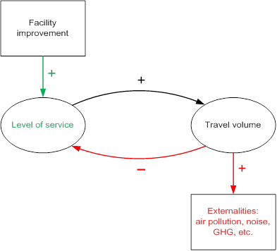
The problem is illustrated in the conceptual diagram in Figure 9:

Figure 9. Flowchart. Effects of a facility improvement on level of service, travel volume, and externalities.

(Source: Cambridge Systematics, Inc.)

• A change is made to a facility that improves level of service (inverse of travel cost) on the facility.
• Improved level of service on the facility encourages higher travel volume on the facility.
• Higher travel volume on the facility in turn reduces level of service on the facility.
• Higher travel volume also results in higher externality costs such as air pollution, noise, and greenhouse gas emissions.

Most transportation analyses today are based on forecasts from traditional four-step travel models, which presume fixed trip-rates regardless of the cost of travel. Hence, changes in demand due to changes in travel costs are not accounted for in the estimation of social benefits and costs. This raises the following issues for analyzing the impacts and social benefits and costs of facility improvements:

• What is the magnitude of induced demand due to a facility improvement?
• How can induced demand – i.e., new trip making due to reduced travel costs – be distinguished from estimated changes in travel volumes due to shifts in route, mode, destination, and time of travel?
• Will induced demand affect facility operations and thereby reduce level of service below that which was originally forecast?
• What are the secondary effects of a facility improvement other transportation facilities in the area, and how can these be accounted for?
• Are current analysis tools capable of accounting for induced demand? If not, are there any quick fixes that could be put in place without substantially changing the regional travel model?

For purposes of this discussion we define induced demand as additional travel due to improvements on a facility that lower the total cost of travel: i.e., additional travel that would not have taken place in absence of the improvements. This is to be distinguished from observed volumes on the facility where the improvements are made, which may be due to one or more of the following:

• Route choice: additional traffic diverted from alternate routes.
• Mode choice: traffic diverted from alternate modes.
• Travel time choice: traffic diverted from alternate time periods.
• Additional travel: new trips made because the total cost of travel is lower.

Of these, the first three could justifiably called apparent (as opposed to real) induced demand; only the last is truly induced demand. As discussed below, the estimation of benefits requires a broader perspective than the particular facility in question. Otherwise, the calculation of user benefits may be biased upward by including apparent induced demand. That is, an improvement on a facility may attract trips that were formerly using more congested routes. Regardless of how demand shifts are characterized, the most important aspect is how systemwide VMT and system operating conditions change as a result of an improvement.

The limited analysis presented here of additional trip making due solely to a reduction in the cost of travel. There are a number of potential effects that can lead to additional induced demand; the most important effect is demand added by increased land development in response to lower travel costs. But it is still common practice in regional travel demand forecasting to use a fixed future land use scenario regardless of changes to the transportation network. Accounting for indirect effects on demand due to changes in land development, though potentially important, is beyond the scope of this project.

Induced Demand in the Context of User Benefits

Real-world estimation of user benefits can be confounded by the following.

Failure to account for systemwide effects. Improvements to a facility can lead to shifts in travelers’ routes, modes, destinations, and time of day of travel. This will show up in travel modeling as increased travel volume on the facility where the improvement is made. But this increase includes effects of travelers who change route and travel mode in response to the reduced travel time. If the increase in volume is attributed solely to new travelers, the benefits to these new travelers will be undervalued by the extent to which the “new” travel volumes on the facility include existing travelers who formerly used other routes or modes, or traveled to other destinations.

Limitations of existing travel models. In economic theory, the demand curve is shown as sloping downward and to the right: i.e., as the price decreases, the quantity demanded increases. But most travel models in use today are four-step models that assume fixed trip generation rates for each purpose; total trip making is insensitive to changes in travel cost. In other words, the demand curve is assumed to be vertical (zero elasticity). While this may be a reasonably close approximation to work trip making in the short run, it is highly implausible for nonwork trips. New generation tour-based travel models that explicitly take into account the dependence of trip generation on travel cost show a that trip making has a significant nonzero elasticity.

There are two ways to address this problem: 1) use a tour-based model that explicitly models dependence of trip making on travel time, or 2) use an independent set of travel demand elasticities to approximate the change in total travel in response to the change in travel time. Table 6 shows a set of travel time elasticities and cross-elasticities derived from simulations using a tour-based travel demand model (Dowling Associates, 2005). Short-run elasticities for truck travel are probably quite small, as these are dependent primarily on economic activity at the trip ends; hence, induced demand for truck travel can probably be ignored for the short run.

Table 6. Travel time elasticities from a tour-based travel demand model.

Demand	Travel Time – AM Peak – Drive Alone	Travel Time – AM Peak – Shared Ride	Travel Time – AM Peak – Transit	Travel Time – PM Peak – Drive Alone	Travel Time – PM Peak – Shared Ride	Travel Time – PM Peak – Transit
AM Peak – Drive Alone	-0.225	0.030	0.010	-0.024
AM Peak – Shared Ride	0.037	-0.303	0.032		-0.028
AM Peak – Transit	0.036	0.030	-0.129			-0.007
PM Peak – Drive Alone	-0.124			-0.151	0.015	0.005
PM Peak – Shared Ride		-0.109		0.019	-0.166	0.016
PM Peak – Transit			-0.051	0.018	0.015	-0.040
Off Peak – Drive Alone	-0.170			-0.069
Off Peak – Shared Ride		-0.189			-0.082
Off Peak – Transit			-0.074			-0.014

Source: Portland Tour-Based Model applied to Puget Sound region (Dowling Associates, 2005).
Note: Blank entries indicate where cross-elasticities were set a priori to zero.

Single set of land use and demographic forecasts. In practice, most regional travel model forecasts are carried out using a single set of land use and demographic forecasts. But land use in particular is sensitive to travel costs.

Other Societal Costs Due to Induced Demand

Externalities due to induced demand include noise, air pollution, and greenhouse gas emissions. Noise effects are still debated, although available studies indicate that a reasonable figure for noise costs are between 0.1 cents and 0.3 cents per mile for freeway traffic (Victoria Transportation Policy Institute). Small and Kazimi (1995) estimated the cost of automotive air pollution at $0.20 per mile in urban areas (Original estimate converted to 2011 dollars). For greenhouse gases, the U.S. Government in 2010 adopted a figure of $21 per ton of CO₂ equivalent, which equates to about 0.8 cents per mile for a fleet average MPG of 25. This has been criticized by some economists as too low (Ackerman and Stanton, 2010); the UK government has estimated short-to-medium term costs of CO₂ at about $87 per ton, or about 3.3 cents per mile (United Kingdom Department of Energy and Climate Change, 2010). In 2013, the U.S. figure was updated to $37 per ton (Technical Update of the Social Cost of Carbon for Regulatory Impact Analysis and Refining Estimates of the Social Cost of Carbon).

Taking the Small and Kazimi estimate for air pollution, the average estimate for noise, the and adding in the official U.S. Government number, this works out to about 20.8 cents per mile for combined externality effects. If these values are used to estimate the externality costs of induced demand, then the externality costs for induced demand for the add-a-lane alternative are about 9 percent to -12 percent of the estimated user benefits, and more than an order of magnitude greater than the additional user benefits due to induced demand.

Case Study: Signal Timing Improvements on an Arterial

Setting

We selected a section of El Camino Real (California State Highway 82) a major arterial in the Bay Area to investigate the induced demand implications for estimating the impacts of common traffic operations improvements. The study section parallels the U.S. 101 study corridor and is often used as an alternative route by commuters. The study section includes 15 signalized intersections for a total length of 3.24 miles. There are three through lanes plus exclusive left turn lanes on all intersection approaches. All signals are coordinated actuated and most of them have protected left turn phases.

We used the SYNCHRO software to evaluate existing conditions and optimize the signal settings (cycle length, splits, and offsets). We checked the baseline conditions and made adjustments to the existing signal settings to eliminate severely oversaturated movements. This is because SYNCHRO (as well as any other signal timing optimization software) cannot accurate model the delays and other impacts in oversaturated conditions, which results in unrealistic improvements during the signal optimization process.

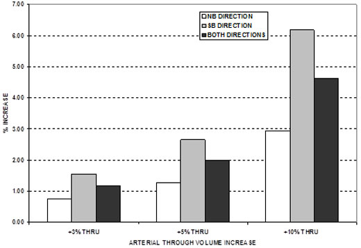
We applied SYNCHRO first to optimize the signal settings under baseline conditions. Next we kept the signal settings fixed and simulated the effects of increased through traffic volume on the arterial by 3 percent, 5 percent, and 10 percent. The results are shown in Table 7 and Figure 10.

Table 7. Estimated performance measures for base case and alternatives.

Performance Measure	Baseline	Baseline Optimal Settings	Induced Demand 3 percent (Percent increase of through volume.)	Induced Demand 5 percent (Percent increase of through volume.)	Induced Demand 10 percent (Percent increase of through volume.)
Arterial Through Traffic – Travel time (sec)	691	589	596	601	617
Arterial Through Traffic – Delay (sec⁄veh)	223	122	128	133	149
Arterial Through Traffic – Vehicle miles of travel	7,579	7,579	7,807	7,958	8,337
Arterial Through Traffic – Vehicle hours of travel	444	378	395	405	435
Arterial Through Traffic – Mean vehicle speed (mph)	17.1	20.0	19.8	19.6	19.2
Arterial Through Traffic – Person miles of travel (Vehicle occupancy of 1.2 person⁄vehicle was assumed.)	9,095	9,095	9,368	9,550	10,005
Arterial Through Traffic – Person hours of travel	532	454	473	486	522
Total System – Vehicle miles of travel	8,879	8,879	9,105	9,257	9,635
Total System – Vehicle hours of travel	515	456	471	481	509
Total System – Person miles of travel	10,655	10,655	10,926	11,108	11,562
Total System – Person hours of travel	618	547	565	13,330	611
Total System – Fuel consumption (gallon)	699	614	632	644	677
Total System – CO emissions (kilogram)	48.9	42.9	44.2	45.0	47.4
Total System – NOx emissions (kilogram)	9.5	8.4	8.6	8.8	9.2
Total System – VOC emissions (kilogram)	11.3	10.0	10.2	10.4	11.0

Figure 10. Bar graph. Change in arterial through traffic travel times.

(Source: Cambridge Systematics, Inc.)

The assumed volume increase of 3 percent is consistent with the reported elasticities in Table 6. Signal timing optimization resulted in 15 percent travel time improvement which could result in induced demand of about 3 percent. We also tested 5 percent and 10 percent volume increases to test the sensitivity of the results.

Analysis Results

Table 7 shows that signal timing optimization with baseline volumes improved travel time on the arterial by 15 percent (from 691 seconds to 589 seconds). The performance was worsened with the induced demand but is still better than the baseline conditions. As Figure 10 shows a 3 percent increase in volumes worsens performance by only 1.2 percent; even a 10 percent increase in through volumes has a better performance than baseline conditions with existing signal settings (Table 7). Note that this type of analysis could be also used to evaluate how much additional traffic can be absorbed by arterial parallel to freeways.

User Benefit Calculations

We used the a value of time ($13.94/hour) for these calculations. We estimated the benefits for a) the baseline conditions with optimal signal settings, and b) induced demand of three percent for through traffic on the arterial. The results are shown in Table 8. Note that these benefits apply only for the AM peak hour. The annual benefits for the AM peak period would be $493,500 for the baseline and $477,500 for the induced demand case assuming 250 weekdays and two hour AM peak period.

Table 8. User benefits.

Performance Measure Total System	Baseline	Baseline Optimal Settings	Induced Demand 3 percent
Person miles of travel	10,655	10,655	10,926
Person hours of travel	618	547	565
Mean person speed (mph)	17.2	1.5	19.3
Travel cost (dollars/person mile)	$0.81	$0.72	$0.72
User benefits		$987	$955

Note that the benefits gained by new users of the facility (induced demand) are not included in the above performance table. However, as pointed out earlier, the benefits to new users (3 percent of all future users) would be approximately one-half of those experienced by current users (97 percent of the future users). Thus, accounting for the benefits experienced by new users (induced demand) would increase the computed benefits (after induced demand) by about 1.5 percent, from $955 to $970. The difference between the computed induced demand benefits and the baseline benefits is $17, less than 2 percent of the computed baseline benefits.

Summary and Conclusions

Several conclusions can be drawn from this analysis:

• The major conclusion is that user benefit calculations must be done at as broad a scale as possible. Estimating user benefits at a facility level only will distort user benefit calculations because the estimates will be confounded mainly by route shifts. The issue of using an appropriately broad scale of analysis appears to be much more significant than whether or not to include induced demand in the analysis.
• There is a benefit to induced travel due to lower travel costs, namely the value of travel to persons who would not have otherwise traveled but are now traveling because of reduced travel costs.
• Induced travel can be estimated at a systemwide level by applying elasticities derived from other studies. While this approximation may not be as good as travel demand estimates derived from a model that specifically incorporates travel cost in trip generation, travel demand elasticities are low enough so that there is little distortion using elasticities alone.
• The case studies estimated that induced demand contributes less than one percent to total demand. Hence, it is unlikely that estimated travel times would change very much if induced demand were included in the operations analysis, even after accounting for the fact that under congested conditions travel times rise nonlinearly with volume increases.
• From the case studies shown here it is clear that benefits to new users are de minimis compared to benefits to current users. This is because: 1) demand elasticities are low to begin with, and 2) the average value of time for new users is about half that of current users. Using the travel time elasticity measures derived in the NCHRP study (Dowling, Richard et al., “Predicting Air Quality Effects of Traffic-Flow Improvements: Final Report and User’s Guide,” National Cooperative Highway Research Program Report 535, 2005) it is clear that even a 10 percent reduction in travel times from the base case would result in at maximum a 3 percent change in demand; such large changes in travel time are not likely in absence of massive capacity increases.
• Externality costs due to induced demand can be significant, and appear to be much higher than benefits due to induced demand. But these still appear to be relatively small (on the order of 10 percent) compared to user benefit estimates.
• The findings from the signal retiming study indicate that induced demand does not significantly affect the system performance under the optimized timings. Also, although we assumed a range of additional traffic (up to 10 percent) in most cases the additional induced demand would be small. Signal timing optimization results in significant 15 percent reduction in travel times, which translates to only about 1.7 minutes savings per traveler at the study corridor.

Effect of Accessibility on Land Use Patterns

Overview

For over 15 years the transportation land use literature has attempted to relate the demand for travel to aggregate measures of the built environment. Models of travel behavior regress an outcome variable – often trip generation, mode choice, or vehicle miles traveled (VMT) – on demographics and measurements of land use. Land use variables are typified by the 3Ds (Kockelman and Cervero, 1997) (Kockelman, Kara, and Robert Cervero. “Travel Demand and the 3Ds: Density, Diversity, and Design.” Transportation Research Part D: Transport and Environment 2, no. 3 (1997): 199‑219) which capture in turn the density, diversity, and design of a geographic area. (Other “Ds” have since been added including destinations, distance to transit, demographics, and travel demand management, e.g., parking. An updated version of the Ds is described in Cervero and Ewing (2010) and a review of the impact of demographics is provided in Pucher and Renne (2003).) Variables commonly include residential density, diversity of land uses, and design of the street grid, and counts of destinations within a constant time distance (an isochrone). Most studies compute land use variables at a fairly coarse geographic scale such as transportation analysis zones (TAZ) or census tracts, despite the fact that the built environment often changes on a block-by-block basis.

This paper added to previous research by proposing and implementing a concept of land uses located in space relative to a multimodal transportation graph, which enables the following contributions to the travel literature. First and foremost, the framework described here is designed to accurately represent pedestrian-scale accessibility, which continues to be a secondary consideration in current travel modeling practice. Second, it has been theorized (Crane, 1996; (Crane, R. “The Influence of Urban Form on Travel: An Interpretive Review.” Journal of Planning Literature 15, no. 1 (2000): 3–23.) Krizek, 2003 (Krizek, K. J. “Neighborhood Services, Trip Purpose, and Tour-based Travel.” Transportation 30, no. 4 (2003): 387–410)) that pedestrian demand cannot be measured accurately without also measuring the relative accessibility of auto travel – indeed some have said that reducing level of service on roads is necessary to induce pedestrian travel (Chatman 2008). (Chatman, D. G. “Deconstructing Development Density: Quality, Quantity and Price Effects on Household Non-work Travel.” Transportation Research Part A: Policy and Practice 42, no. 7 (2008): 1008–1030.) Finally, 3Ds variables are criticized on the grounds that they do not propose a behavioral explanation for travel (Boarnet and Crane, 2001) (Boarnet, M., and R. Crane. Travel by Design: The Influence of Urban Form on Travel. Oxford University Press, USA, 2001). This paper takes the position that travel is a derived demand most heavily influenced by access to destinations, traits of the routes to those destinations, and modified by attributes of the decision-maker (e.g., Cervero, 2002 (Cervero, R. “Built Environments and Mode Choice: Toward a Normative Framework.” Transportation Research Part D: Transport and Environment 7, no. 4 (2002): 265–284); Guo et al., 2007 (Guo, Jessica Y., Chandra R. Bhat, and Rachel B. Copperman. “Effect of the Built Environment on Motorized and Nonmotorized Trip Making: Substitutive, Complementary, or Synergistic?” Transportation Research Record: Journal of the Transportation Research Board 2010, no. -1 (2007): 1–11)).

A number of methodological advances enable this research, which allows representation of the full set of local streets for pedestrian-scale accessibility, a hierarchical graph to capture the tradeoff between modes, and integration of microscale land use data to measure the full population of alternative destinations in the city. A fully estimated destination choice model is beyond the scope of this project due to length requirements, but future research will address this question fully.

We examined the question of whether and to what degree policies which encourage compact development can reduce VMT and the concomitant greenhouse gas (GHG) emissions (Boarnet, 2011 (Boarnet, M. G. “A Broader Context for Land Use and Travel Behavior, and a Research Agenda.” Journal of the American Planning Association 77, no. 3 (2011): 197–213); Brownstone, 2008 (Brownstone, D. “Key Relationships Between the Built Environment and VMT.” Transportation Research Board (2008): 7)). This topic is of particular relevance in the State of California, which has passed Senate bill 375 (SB375) which mandates that each of its MPOs creates a sustainable community strategy (SCS). Each SCS must analyze potential GHG reduction through coordinated land use and transportation (Barbour and Deakin, 2012) (Barbour, Elisa, and Elizabeth A. Deakin. “Smart Growth Planning for Climate Protection.” Journal of the American Planning Association 78, no. 1 (2012): 70-86), and must model the impact of policies which increase residential density on reductions in automobile use and increases in travel by sustainable modes such as walking, bicycling, and public transit. This research is performed as part of the UrbanSim (Waddell, 2002) (Waddell, P. “UrbanSim: Modeling Urban Development for Land Use, Transportation, and Environmental Planning.” Journal-American Planning Association 68, no. 3 (2002): 297-314) analysis performed by the Urban Analytics Lab at UC Berkeley for the San Francisco Bay Area SCS funded by the Metropolitan Transportation Commission (MTC).

Previous Research

For over 15 years the transportation land use literature has attempted to relate the demand for travel to aggregate measures of the built environment. Models of travel behavior regress an outcome variable – often trip generation, mode choice, or vehicle miles traveled (VMT) – on demographics and measurements of land use. Land use variables are typified by the 3Ds (Kockelman and Cervero, 1997)(Ewing, R., and R. Cervero. “Travel and the Built Environment: a Synthesis.” Transportation Research Record: Journal of the Transportation Research Board 1780, no. -1 (2001): 87-114), which capture in turn the density, diversity, and design of a geographic area. Variables commonly include residential density, diversity of land uses, and design of the street grid, and counts of destinations within a constant time distance (an isochrone). Most studies compute land use variables at a fairly coarse geographic scale such as transportation analysis zones (TAZ) or census tracts, despite the fact that the built environment often changes on a block-by-block basis.

Despite limited microdata available at the time, Ewing and Cervero (2001) are able to draw broad conclusions based on a wide breadth of empirical literature that trip generation is largely based on demographics, trip distance varies largely with the built environment, and mode choice depends on both demographics and the built environment, but predominantly on demographics. Although these early studies were a major contribution to our understanding of the influence of land use on the demand for travel, this type of study was quickly criticized for its lack of behavioral foundation (Crane, 2000; Boarnet and Crane, 2001). Boarnet (2011) identifies 3Ds-style studies as “reduced form” models and argues for the move to “structural models,” which explain why residential density, for instance, might influence travel.

Pedestrian Models

Data has become increasingly available at the pedestrian-scale, and a large body of literature in the demand for pedestrian travel has resulted. The commercial success of Walkscore, which now services almost six million queries a day, is well established. Walkscore is a weighted combination of the fine-grained location of nine types of nearby destinations (Walkscore, 2011) (“Walk Score Methodology.“ Front Seat, Inc., July 15, 2011.); its raison d’etre at this time as a commercial application is in selling real estate and the correlation with real estate values has been established (Copyright 2009) (Copyright, Joe. “Walking the Walk: How Walkability Raises Home Values in U.S. Cities” (2009). Crane, R. “On Form Versus Function: Will the New Urbanism Reduce Traffic, or Increase It?” Journal of Planning Education and Research 15, no. 2 (1996): 117&8209;126).

Recently, Walkscore has been confirmed as predictive of walking trip generation (Weinberger and Sweet, 2012) (Weinberger, Rachel, and Matthias N. Sweet. “Integrating Walkability Into Planning Practice.” In Transportation Research Board 91^st Annual Meeting, 2012) but this study relates Walkscore to modeled pedestrian outcomes derived from travel models, which themselves misrepresent the walking environment. The theoretical framework established for Walkscore in Frank et al. (2008) (Frank, L. D, J. Kerr, J. F Sallis, R. Miles, and J. Chapman. “A Hierarchy of Sociodemographic and Environmental Correlates of Walking and Obesity.” Preventive Medicine 47, no. 2 (2008): 172-178) and Moudon et al. (2006) (Moudon, A. V, C. Lee, A. D Cheadle, C. Garvin, D. Johnson, T. L Schmid, R. D Weathers, and L. Lin. “Operational Definitions of Walkable Neighborhood: Theoretical and Empirical Insights.” Journal of Physical Activity & Health 3 (2006): 99 is likely valid, but the set of destinations, the weights applied to the destinations, and the distance decay function are empirical questions that merit more investigation. Additionally the relationship of pedestrian travel to meso- and macroscale accessibility is largely missing from this line of research.

Econometric Frameworks

Econometric frameworks have long been the workhorse of travel modeling. Discrete choice modeling (McFadden, 1980) (McFadden, D. “Econometric Models for Probabilistic Choice Among Products.” Journal of Business (1980): 13-29) allows the estimation of indirect utility among a discrete number of alternatives subject to a linear in parameters utility function and a given distribution for a random error term. Discrete choice was first widely applied to travel demand models by Ben-Akiva and Lerman. A framework for mode choice is provided in Cervero (2002), which allows for both discrete choice estimation of utility among travel modes as well as using 3Ds measurements as explanatory variables. This approach is used in Guo et al. (2007), which studies the substitution of pedestrian and auto modes, finding that pedestrian travel is largely complimentary to automobile travel (in other words, pedestrian access generates additional walking trips that do not tend to substitute for automobile travel).

The City in a Network

First and foremost, it is presumed that travel is a derived demand such that there is an “attractor” at the destination which is counteracted by an “impedance” in the network as is typical of the gravity model (Hansen 1959). (Hansen, W. G. “How Accessibility Shapes Land Use.” Journal of the American Institute of Planners 25, no. 2 (1959): 73-76. Measurements include “isochrones” which sum opportunities within a distance or travel time, “gravity model” measures which discount the opportunities by some measure of the distance to each destination, and logsum measures which estimate coefficients on attractors and impedances using a statistical framework, typically using a discrete choice model.) Unlike the gravity model, this network-based model estimates the relative importance of attributes which can include 1) the amount or quality of activity at the destination; 2) aspects of the route; and 3) attributes of the decision-maker, which modify the elasticities of the first two sets of traits.

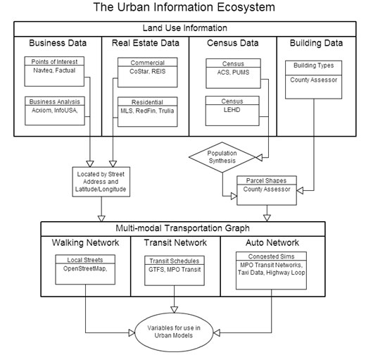
The simplest version of the conception proposed here places land use in the context of the local street network, using network distances that are equivalent to the length of the streets traversed. Most urban spatial data is either georeferenced with a latitude and longitude or is assigned to a parcel and thus has a spatial position through the location of parcels in a region. (There are currently around 150 million non-government owned parcels in the United States (another 10 million are owned by the government). The primary purpose of parcels is two-fold: preventing/resolving private property disputes between land owners and efficient collection of property taxes.) A typical schema of urban data relationships is shown in Figure 11, which depicts data frequently used in urban modeling (e.g., Waddell 2002): households and businesses are assigned to buildings which are assigned to parcels which are placed within the context of the local street network. Alternatively, any spatial data can be assigned to the network by latitude or longitude or any other geometry representable in a geographic information system (GIS). Figure 11 describes the land use and transportation datasets used in this research. Each box is a dataset with the type of data above and the possible sources listed inside the box. Relationships between land use and the transportation network are mediated either through a latitude/longitude pair or a parcel shape which defines a location in the city.

Figure 11. Flowchart. Interaction of information in an urban system.

(Source: Waddell, P. “UrbanSim: Modeling Urban Development for Land Use, Transportation, and Environmental Planning.” Journal of the American Planning Association 68, no. 3 (2002): 297-314.)

Assignment of Land Use

Land use data must be efficiently connected to the transportation network. Datasets are large, and the number of objects of each type for the Bay Area implementation is shown in Table 9. In an ideal case, the synthesized population and dataset of firms are assigned to the parcel map, and the parcel map gives addresses that define the means of access and egress from that parcel to the local street network. Every person has access to every firm and vice versa via these access and egress points. This complete graph of parcel connections is here called the Parcel Graph.

In practice, data currently are subject to a complicated set of messy interrelationships. Although population might be accurate at higher-level census geographies, the assignment to buildings is typically performed by iterative fitting to observed marginals (Beckman et al., 1996) (Beckman, R. J, K. A Baggerly, and M. D McKay. “Creating Synthetic Baseline Populations.” Transportation Research Part A: Policy and Practice 30, no. 6 (1996): 415-429), which introduces error. Firm data is yet more problematic: establishments are tracked in a number of datasets, but businesses with multiple locations are often assigned to a single building, and geographic knowledge is often no more specific than assignment to the nearest tract or block group centroid. Building data are maintained by county assessors and contain myriad errors in spatial encoding, including repeated stacked or overlapping parcels, misrepresentation of buildings types, unrecorded informal units, etc.

Table 9. Number of objects per dataset used in the Bay Area SCS implementation.

Object	Count of Objects
Parcels	2,023,915
Single Family Houses	1,479,511
Non-SF Buildings	456,749
Establishments	464,302
Jobs	3,395,967
Households	2,608,023
People	6,996,929

Street Node Geography

An extremely useful simplifying assumption has been made in this research to adopt “street node geography.” In this case, each land use is mapped to its nearest street intersection and thus all land use is assumed to exist at point locations coincident with the vertices of the network being used, here called the Node Graph. Thus, the city can be conceived as a Voronoi diagram of the local street network intersections. Spatial data is assigned first to parcels, parcel centroids are mapped the nearest street node, and the relationship between parcels and nodes is used to map land use to the network. (A dual conception exists here where land use is mapped to the nearest edge as opposed to the nearest vertex. This is “block face” geography (Clifton et al. 2008) and can be represented by using the “line graph” of the local street network in which every edge is replaces by a vertex and vice versa. Block face geography can be more accurate than street node geography in some situations: for instance, real estate value and demand might vary by block face rather than street intersection.) Since walking distances are typically significantly larger than the distance from each parcel to its nearest street intersection, this reduces accuracy of models very little.

Additionally, street networks are an immanent and varying property of cities which are naturally denser in the dense areas of the city and sparser in less dense areas of the city. Thus, the street network is an important cue that there is less information present in areas which have large distances between nodes, and the street network “compresses” the city appropriately. Space is thus represented more accurately where it matters most. (This assumption fails for large parcels like urban parks, university campuses, and corporate office parks. Generally speaking, where location of actual buildings is known, assignment of building to street node directly should be done. Unfortunately, this information is often unavailable and large parcels must be allocated proportionally to all adjacent street nodes.) This reduces the number of land use elements by almost a factor of 10 which relieves computational burden while maintaining spatial resolution appropriately. The assignment of land use can be applied to any network, including networks for other transportation modes discussed next.

You may need the Adobe® Reader® to view the PDFs on this page.