Guide for Highway Capacity and Operations Analysis of Active Transportation and Demand Management Strategies
Appendix M: The Equilibrium Effects of ATDM
The equilibrium effects of ATDM come into play as travelers on other facilities in the area recognize the time and reliability savings of the ATDM improvements on the subject facility and shift their route choice, time-of-day choice, and their mode choice to take advantage of the improved operations on the subject facility. This effect may be called by some, “induced demand.”
For the purposes of estimating the benefits of ATDM investments it is not strictly necessary to account for the equilibrium effects of ATDM, because travelers drawn to the facility from other facilities (or modes or times of day) do so because they also experience a net benefit from the ATDM improvements to the subject facility. In addition, their leaving the other facilities also improves the operation of the other facilities for those drivers remaining on the other facilities.
Accounting for the equilibrium effects of ATDM is important when one wishes to obtain a more accurate estimate of facility performance after drivers in the area have adapted to the improved conditions.
Overview of Equilibration Process
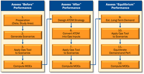
The steps of the equilibration process are as follows (also see Figure 11):
- Estimate Long-Term Demand Shifts: Shifts in demand (destination choice, mode choice, time-of-day choice and route choice) are estimated based on the predicted percentage change in mean travel time, mean travel cost, and travel time reliability caused by the ATDM strategy.
- Apply Operations Analysis Tool to Scenarios (Long-Term): The same operations analysis model is applied using the new demand estimates to compute performance.
- Equilibrate Demand and Performance: The change in travel time predicted with the new demands is compared to the change in Opening Day travel times which was used to predict the new demands. The estimated new demand values are equilibrated until they no longer change significantly between iterations.
- Compute MOEs (Long-Term): The results output by the operations analysis tool for long-term, after equilibration of the new demands, are combined to yield the desired MOEs. The analyst assesses the long-term performance results and decides if the ATDM strategy needs to be fine-tuned and reanalyzed.
Figure 11: Flow Chart of ATDM Analysis Process – With Equilibration

Source: Cambridge Systematics, Inc.
Step 9: Estimate Long-Term Effects
The six-month effect of ATDM on facility performance (after travelers have had a chance to adjust to the improved conditions) is determined by computing the effect of the facility performance improvements on demand. The revised demand is used to reestimate the travel times with ATDM. The revised travel times and demands are iterated until a new equilibrium is achieved.
Highway capacity and operational improvements, including ATDM strategies, will affect demand by improving travel times. It is important to consider the demand effects when evaluating the environmental impacts of capacity and operational improvements. It is especially important for evaluation of ATDM strategies because they explicitly seek to control demand so as to improve system operating efficiency.
In the context of highway operational improvements such as those associated with ATDM, long-term is considered 5 to 6 months after the operational and/or capacity improvements have been implemented. Travelers have had sufficient time to become accustomed to the new facility travel times and have adjusted their behavior (start times, destinations, modes, and routes) to take advantage of the new conditions.
The long-term demand effects are best estimated using a regional travel demand model, but this can frequently be impractical when conducting facility-specific studies. In addition, regional demand models often have difficulty accurately representing congested conditions on highways and the effects of operational improvements. A sketch planning model approach is consequently provided for when it is not feasible to use a regional demand model.
The forecasted new demands must be equilibrated with the demands used to estimate the travel times until the differences between the demands used to estimate the travel times, and the demands estimated from the travel times are negligible.
Overview of Long-Term Demand Method
The Opening Day demands and travel times are compared to the “Before” demands and travel times. An estimated long-term demand is produced. The estimated long-term demand is compared to the opening day demand. If the two demands are sufficiently different the HCM method is applied to the long-term demands to obtain long-term travel times and the new travel times used to produce a second estimate of the long-term demand. These computations are repeated until equilibrium in the demand estimates is achieved. The last iteration travel time and demand estimates are reported out as the long-term performance of the facility with highway capacity and/or operational improvements.
Utilization of Regional Demand Models
Regional demand models devote a great deal of effort to predict travel demands over the large geographic areas necessarily to fully capture travel behavior. As a consequence, regional demand models sacrifice accuracy and precision in the modeling of the traffic operations of individual segments of individual highway facilities.
If a regional demand model is to be used to model the demand effects of capacity and operational improvements it is necessary to integrate the demand model with a traffic operations model of sufficient precision to accurately model the traffic operations effects of the capacity and operational improvements. The two models must then be equilibrated to ensure that the travel times used to estimate the demands in the demand model are the same as the demands used to estimate the travel times in the traffic operations model.
The integration and equilibration of two models can be quite resource-intensive, thus an alternative sketch planning approach to demand modeling is presented in the next section. The full regional demand modeling approach will provide the more comprehensive and reliable estimates of demand changes; however, when it is not feasible to apply the full demand model, a sketch planning approach is much superior to assuming that demand does not change at all.
Sketch Planning Methodology
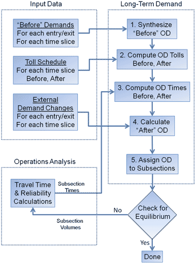
An overview of the sketch planning methodology for estimating long-term demand is presented in Figure 12. The origin-destination (OD) table for the facility is estimated from the segment flows. The facility toll schedule (if any) is converted to the equivalent OD toll table. The facility segment travel times are converted to OD travel times. The differences between the before and after travel times and tolls are used to estimate the new OD table of demands. The new demands are assigned to the appropriate facility segments. The new “after” demands are compared to the “before” demands. If they are within the specified closure criteria, the analysis is complete. If not, then the operations analysis tool is used to recompute the facility segment travel times using the new demands. The new “after” travel times are fed back to the demand module. The process is repeated until the change in demands drops below the closure criteria.
Figure 12: Sketch Planning Model Flow Chart

Source: Cambridge Systematics, Inc.
Step 9.1: Synthesize Facility OD Tables
The facility section demands must be converted to origin-destination (OD) table of demands for the facility. This is necessary so that each vehicle’s entire trip experience on the facility is accounted for in evaluating changes in demand.
If HOV lanes are to be evaluated, then separate OD tables should be constructed for HOVs and for SOVs.
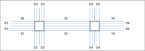
Figure 13 and Figure 14 illustrate origin-destination numbering schemes for a typical freeway and a typical street. A freeway may be evaluated one direction at a time when generating the OD table. An arterial street must be evaluated for both directions of travel when generating the OD table.
The OD table for each time slice (and each mode – HOV, SOV) within the scenario is estimated based on the entry and exit demands for the facility and the relative distance between the two points.
Equation 17
Where:
Tij = Vehicle-trips entering facility at origin “i” and exiting at destination “j.”
Ti = Vehicle-trips entering facility at origin “i.”
Tj = Vehicle-trips entering facility at destination “j.”
L(ij) = the distance in feet between origin “I” and destination “j”
f(ij) = distance weighting factor.For Arterials:
f(ij) = 1 for all i<> j
f(ij) = 0 for all i = j (assume no U-turns)For Freeways:
f(ij) = exp(-4/L(ij)) for “j” = off-ramp
f(ij) = 1 for “j” = mainline out
For freeway facilities under 5 miles in length one might assume that the ramp to ramp OD demands are small enough that they can be neglected. In this case, then 100% of the on-ramp demands go to the mainline destination, and 100% of the off-ramp demands come from the mainline origin. Of course, if the analyst has information on specific local circumstances causing significant on-ramp to off-ramp demands, then that information should be employed in the construction of the facility OD table by time slice.
Figure 13: Example Freeway Facility Origins and Destinations

Source: Cambridge Systematics, Inc.
Key: O1 = Origin #1; D1 = Destination #1; S1 = Directional Section #1
Figure 14: Example Street Origins and Destinations

Source: Cambridge Systematics, Inc.
Key: O1 = Origin #1; D1 = Destination #1; S1 = Directional Section #1
Step 9.2: Convert Schedule of Tolls to OD Tolls
The schedule of tolls for the facility or HOT lane (if any) is converted to the equivalent origin-destination toll for the facility for each time slice.
Step 9.3: Compute OD Travel Times
The facility section travel times are summed up to obtain facility origin-destination (ODODplies full trip elasticities.
Step 9.3A: Convert Segment Travel Times to Facility OD Travel Times
The facility section travel times are summed up to obtain facility origin-destination (OD) travel times. If there are multiple paths to a destination, then the travel times for the shortest travel time path are summed.
For the purpose of computing the shortest travel time path, tolls, if any, are converted to the equivalent travel time in minutes by dividing the toll by the driver’s value of time (VOT). The value of time can be computed based on average income for the area and using FHWA’s TRUCE program. Values of Time for selected large urban areas are provided in Table 49.
Source: FHWA TRUCE.
Step 9.3B: Extrapolate Facility OD Travel Times to Complete Trip Times
The facility OD travel times are extrapolated to full trip travel times (sum of on-facility and off-facility trip times). The traveler’s full trip travel time is assumed to be a function of the amount of time they spend on the facility. This computation is applied for each time slice within the scenario.
Equation 18
Where
TT(ij) = Full trip travel time for facility travelers using facility to go from “i” to “j” (min.).
TF (ij) = travel time on the facility for the entry-exit pair (min)
TR (ij) = peak period regional average travel time (min)
Note that when TF is small, average total trip time is approximately equal to the regional average trip time. As TF increases, the average total trip time increases so that travel time off the facility is always greater than zero.
Step 9.3C: Compute Reliability Weighted Trip Times
SHRP 2-L04, Incorporating Reliability Performance Measures in Operations and Planning Modeling Tools, will be addressing the effects of travel time reliability on demand, however, that research will not be completed until February 2012. So for the interim the following equation is recommended to calculate travel time equivalents for a trip:
Equation 19
Where:
TTE = The travel time equivalent on the facility for the entry-exit pair (min)
TT(mean) = The mean travel time (min)
“a” = Calibration parameter (default is 1.00)
TT(80%) = The 80th percentile travel time (min)
TT(50%) = The 50th percentile travel time (min)
Step 9.4: Compute Demand Response
For each time period, entry-exit pair, vehicle class, and lane class, the change in volume due to the change in travel time equivalents is calculated using a mixed power-exponential function.
Equation 20
Where
T0 = The “Before” travel time equivalents (min)
V0 = The “Before” demands (veh)
T = The “After” travel time equivalents (min)
V = The “After” demands (veh)
β = Beta, travel time elasticity (default is -0.2)
γ = Gamma, route diversion parameter (default is 0.0)
This equation is applied three times for each OD pair and time slice: once to nontoll-paying SOVs, once to toll-paying SOVs, and once to HOVs. If HOVs are charged a toll (so that some switch to the HOT lane and some stay in the all-purpose lanes), then it would be applied four times.
The route diversion effects (captured by (Gamma) in the above equation) will vary greatly from situation to situation, depending on the characteristics of alternative routes. If the facility in question is an isolated freeway that operates at speeds much higher than parallel arterials, we would expect route diversion to be minimal (the value of Gamma would be near zero). However, if there are parallel freeways nearby or if the freeway is congested so that its speeds may not be that much greater than parallel arterials, then route diversion could be very significant.
Step 10: Apply Operations Tool
The selected HCM traffic operations analysis tool is applied to the scenarios using the new demands estimated in the previous step. The traffic operations analysis tool is applied separately to each scenario to compute predicted segment travel times for the facility under each scenario.
Step 11: Equilibrate Results
Since the previous step will result in new estimates of travel times for the new demands, it is necessary to equilibrate the results until the predicted demand changes are consistent with the predicted travel time changes used to estimate the demand changes. The equilibration process proceeds as follows:
- For each cell in each OD table for each time slice compute the ratio of the new predicted trips to the opening day predicted trips.
- If the ratio is less than 0.9995 or greater than 1.0005 then:
- Take half the difference between the new predicted trips and the opening day predicted trips and add it to the opening day predicted trips.
- Assign the new demands to the facility sections.
- Reapply the HCM analysis to the new predicted demands.
- Compute new segment mean travel times and 80th percentile travel times.
- Compute new OD travel times (repeat Step 9.3) and recompute new demand (Step 9.4).
- Compare new OD trips to previous iteration estimated of OD trips.
- Stop iterations when ratios of latest iteration to previous iteration trips for each cell of OD tables is within 5 one-hundredths of one percent of 1.00.
Step 12: Compute MOEs (Equilibrated)
Assess Long-Term Performance
The “Long-Term” performance is computed for each scenario using the same procedures as were used for the “before” case.
Adjustments for Congestion Spill Over
In cases where the estimated queues spill over the temporal and/or spatial limits of the operations analysis tool then the best solution is to expand the limits of the tool and rerun the analysis. The limits should be revised if the spillover is frequent, occurring in many scenarios with cumulative probability of greater than 10%.
However, if the cumulative probability of those scenarios with spillovers is less than 10%, then the analyst may consider whether resource constraints, the low probabilities of such extreme scenarios, and cost-effectiveness considerations, may limit the ability to expand the limits. In such situations, it is necessary for the analyst to work with the study stakeholders to:
- Assess the probability (and therefore the significance) of the scenarios causing the overflow,
- Assess the degree to which not accurately modeling the overflows will introduce bias that would significantly affect the decisions regarding ATDM investments, and, if significant,
- Determine if a reasonable increase in the study limits will adequately capture the overflows, and if not,
- Approximately account for the congestion spill over outside of the operations analysis tool limits. Use the methodology described in Section 5.4 (Step 4).
If the decision is made at this late stage in the process that the study limits must be revised, then the “before” and “opening day” analyses will have to be repeated with the new limits so as to produce results comparable with the revised “long-term” analysis study limits.
previous

