Traffic Analysis Toolbox Volume XIV: Guidebook on the Utilization of Dynamic Traffic Assignment in Modeling
8.0 Model Calibration
The objective of transportation model calibration is to properly represent observed field traffic conditions in the model. In the calibration process it is important to understand both the approach and methods for calibration and the end goal of calibration.
DTA models employ a wide range of simulation techniques from different time resolutions to different simulation algorithms. Analysis teams conducting model calibration must have a clear understanding of DTA principles and the DTA methodology within the software. Ideally, the software documentation provides guidance on the model parameters and their impact on the performance of the model. This chapter outlines an approach to calibration of a DTA model independent of the specific software package being used.
This section of the guidebook discusses the following:
- Terminology used in model calibration;
- Software and DTA considerations in calibration;
- An overarching calibration process applicable to any software package;
- Recommended sequence of calibration adjustments; and
- A model calibration checklist.
8.1 Calibration Terminology
For the purposes of this guidebook calibration is defined as a process whereby the analyst selects the model parameters that cause the model to best reproduce field-measured local traffic operations conditions. This process also includes the statistical verification of the model outputs vis à vis the field-measured conditions.
Validation in transportation modeling is often used as the term for verification of the model outputs. Validation in this guidebook is defined as a process in which a calibrated model is tested using a different set of existing traffic data to determine if the calibration parameters are applicable to other conditions.
8.2 DTA Considerations
The analysis team must understand the underlying simulation and modeling techniques in a DTA model in order to understand how the model would react to network and demand changes and the measures of effectiveness that should be the focus of calibration. With this understanding, the analysis team can then make the adjustments so that the simulation results reflect observed conditions.
In calibration of any transportation model, some of the more typical measures used are volumes, speeds, travel time, and congestion (length and duration of queuing). These measures are used in a DTA model as well; however, with DTA there are other measures that require additional attention in calibration, including route choice and trip making by time of day.
The fidelity of a model with DTA depends on more than link volumes. It is important that the trip characteristics (path and time of trip taken) reflect observed conditions and expectations. Increasingly, vehicle path data are becoming available through Bluetooth and GPS technologies, enhancing the ability to accurately assess DTA models.
Model Scale Considerations
Models using DTA tend to cover large areas, and the ability to obtain good calibration data for the entire model may be limited. There are methods of addressing these circumstances. The analysis team may use screen lines and cut lines as a method for capturing trip making in the project area.
Another consideration is dividing the model into a primary and secondary area. The primary area is where the subject of the analysis is located and where the data with the highest fidelity are located. The secondary area is important to the model for network completeness but is outside of direct influence by the mitigation strategies under consideration, and may not have data of the highest fidelity.
8.3 Calibration Process
The general DTA model calibration process is comparable to what has been used for microscopic traffic simulation models and presented in the Traffic Analysis Toolbox Volume III. There are DTA-specific considerations that need to be addressed in the adjustments applied to model components as well as overall model behavior. The overall process for calibration is presented in the following summary list.
- Establish calibration objectives and review project objective to ensure that the calibration task directly supports the project objective.
- Identify the performance measures and critical locations against which the models will be calibrated.
- Determine the statistical methodology to be used to compare modeled results to the field data.
- Determine the strategy for model calibration and identify parameters within the DTA models that are the focus of adjustments.
- Assemble field data previously collected for comparison to model outputs
- Conduct model calibration runs following the strategy and conduct statistical checks. When statistical analysis falls within acceptable ranges, then the model is considered to be calibrated.
- Validation: Test or compare the calibrated model with a data set not used for calibration. If the model replicates the different data set the calibration parameters and model are considered to be validated.
A detailed discussion of each step in the calibration process is presented in the following subsections. Figure 8.1 below depicts a general procedure applicable to calibrating a DTA model.
Figure 8.1 DTA Model Calibration Framework
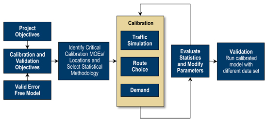
Source: Cambridge Systematics, Inc.
8.4 Establish Calibration Objectives
Model calibration objectives must be consistent with project objectives. Type of project, stakeholder objectives, and model considerations feed into the calibration objectives, as depicted in Figure 8.2. The following example demonstrates how these objectives influence the decision on model calibration objectives:
Example: Near-Term Bottleneck Removal and Prioritization
Agency “A” is preparing to expend a significant portion of its capital funds on a series of bottleneck improvement projects. It has more projects than it has funds. The level of accuracy desired is high because the funds need to be allocated as prudently as possible. The agency has recognized the complexity of the problem and has programmed sufficient funds for data collection, including an O-D survey. The regional demand model has recently been updated and both mesoscopic and microscopic base models are available. The desired operational analysis on the freeway bottlenecks is a microsimulation analysis.
Figure 8.2 Calibration Objective Considerations
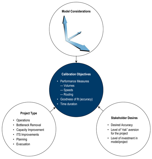
Source: Cambridge Systematics, Inc.
Calibration objectives: The desired level of accuracy (low margin of error) would be high for this project because sufficient data would be available for model development and calibration. The number of measures tested should be expanded to include path making, in addition to traffic volumes and travel speeds.
Overall, model calibration needs to be a well-planned task because it may consume substantial resources if the calibration acceptance targets are not properly and realistically defined upfront.
8.5 Identify Performance Measures
The performance measures used in model calibration are the measures that can be collected in the field and produced by the model software. In the calibration process the field data are compared to the model outputs, and if the calibration acceptance criteria are satisfied, calibration is considered to be complete.
The performance measures for calibration should also be consistent with the performance measures to be used to evaluate scenarios. The analysis team should begin by identifying a set of “must-have” performance measures, then estimate the resource requirements, then gradually include additional “good-to-have” performance measures if budget and schedule allow. Defining all-inclusive and over-ambitious calibration targets often leads to overwhelming resource requirements and execution risk. Calibration and targets should be agreed upon by key stakeholders during the scoping phase.
The collection of performance measurements in the field can be used in developing model calibration acceptance targets. It is important to understand that there are variations and discrepancies in empirical data either because of instrument errors or because of differences in data collection dates. The calibration acceptance targets may need to be adjusted based on the variability observed in the data. There are several documented statistical measures that describe the “goodness-of-fit” of a model in calibration. These include traffic volumes, speeds, travel times, and congestion.
Identify Critical Locations
Bottleneck locations are typically the most important areas to focus on during the calibration process. In arterial street modeling, bottlenecks are typically found at intersections or where road characteristics change resulting in decreased capacity (such as lane reduction, etc.). In freeway modeling, bottlenecks occur in similar locations – where road characteristics change resulting in decreased capacity, and upstream or downstream of interchanges related to weaving and merging traffic. There also are external causes of bottlenecks, such as sight distance variation, vistas, and other driver distractions, that are more difficult to assess but equally important to understand. Understanding the cause of a bottleneck is the first step in calibrating a model to replicate its effects, which is why it is important to develop an existing conditions report.
A summary of the data collection activities should include a description of all the critical locations and important performance measures. The observed values of each measure should be included (e.g., “the maximum queue at each study area intersection is reported in Table X”; “volumes along the freeway and on all freeway ramps can be found in Figure Y”).
Calibration Statistics
Various statistical methods can be used to measure how well a DTA model is calibrated. A model will never be perfect, so the analysis team should identify a level of error tolerance after studying the variability of field data in the real world transportation system to be modeled and the stochasticity of the DTA model. The model should be able to emulate the actual performance in the field and the variability of that performance. Specific examples of statistical approached to this end are provided in Chapter 6 of the Level of Effort Guide. Furthermore, quality and consistency issues may exist in the calibration data set; perfectly matching a set of inconsistent data may be impossible and undesired from a modeling perspective. A calibrated DTA model should consistently reproduce the spatial and temporal characteristics of the local traffic patterns within the specified level of tolerance.
8.6 Calibration Strategy
Model calibration involves adjusting model parameters and inputs to improve the model’s ability to replicate local conditions. This chapter focuses on the calibration strategy for dynamic user equilibrium (DUE) in DTA models irrespective of their simulation resolution: mesoscopic, microscopic, or hybrid. DTA models may differ in their approaches, but their challenge is similar: providing a solution to the DUE problem and using this solution as the basis for equilibrium.
Observed data sets that are statistically significant and provide good coverage of the analysis area are a prerequisite for the calibration process. As presented elsewhere in this guidebook, the objective of building a DTA model is to model the spatial and temporal characteristics of congestion. To calibrate the base-year model, observed data should exist on volumes, travel times, and queues. Counts alone are insufficient, because in DTA models (consistent with traffic flow theory and field observations), the same flow can be observed under congested and uncongested conditions. As a result, a model calibrated against counts only may have limited predictive ability due to the fact that it may not adequately replicate congestion and the associated time-varying travel times that drivers use in making route decisions.
To make calibration practical, a sequential process must be followed in which the traffic flow model is calibrated before the route choice model. This ensures that capacities and the relationship between traffic speed and flows are being modeled accurately. Route choice depends on the time-varying speeds provided by the traffic simulation model. As a last resort and at the concurrence of the analysis team, O-D matrix adjustments may be necessary if during the calibration the accuracy of the input demand is determined to not be adequate. By calibrating both the traffic simulation and the route choice model before adjusting the demand, the analysis team will reduce the need to adjust demands. The recommended sequence and steps in the calibration process is as follows:
- Calibrate traffic flow parameters (capacity and speed-flow relationships);
- Calibrate route choice (software parameters, costs by link, travel time, driver preference, global driver behavior);
- Calibrate temporal O-D matrices including time departure adjustments; and
- Fine-tune (quantitative analysis – adjust local variables to match queues and operations).
Calibrate Traffic Flow Parameters
The following steps are included in this stage:
- Review the model software manuals and guidance about the suggested approach to calibrating relevant attributes in the simulation model;
- Observed data should reflect both the free-flow and congested conditions; and
- Under various simulated density conditions, estimated speeds should correspond to the observed speeds under similar traffic conditions.
Typical statistical metrics determining the goodness-of-fit of the simulated measures can be used such as the linear regression model. Figure 8.3 illustrates how observed and calibrated speeds can be compared.
Figure 8.3 Comparison of Observed versus Model Estimated Speeds
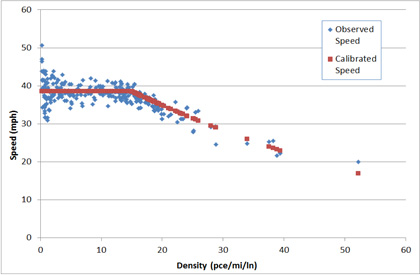
Source: University of Arizona.
Existing simulation-based DTA models adopt a wide range of simulation methodologies, ranging from microscopic to mesoscopic simulation logic rules. Experienced capacity in a simulation model can be estimated based on the simulation logic and how vehicles maneuver based on the underlying car-following and lane-changing models. For instance, the interaction between vehicles and the roadway is influenced by driver aggressiveness, which is ruled by the simulation logic. Attributes such as gap acceptance and reaction time to congestion or controlled-intersections affect the experienced capacity and performance of the simulated roadways.
Calibrate Route Choice
Route choice is a critical component of a DTA model. The route choice model could be implemented in various ways, each based on specific choice behavior assumptions (e.g., dynamic user equilibrium or random utility maximization) and model constructs (e.g., utility functions or generalized cost function). Calibrating the route choice model involves determining the best coefficients of the variables in the utility function or cost function. In calibrating route choice the settings on how drivers respond to roadway attributes and congestion and to changes in the transportation system are established, which affects the modeled link volumes and speeds.
For example, if there is a bias in the study area towards continuous flow facilities such as freeways, then the route choice model should be calibrated to reflect differing weights of travel times associated with different types of facilities. The goal of the adjustments is to more realistically reflect the true route choice behavior.
Once the traffic simulation model is able to reproduce traffic flow streams with the proper characteristics such as capacity and speed, the analysis team should turn their attention to the calibration of the route choice model. The most important parameters affecting route choice are travel time, link-based cost, distance, functional class, number of turns, and percentage of time not moving. Assigning the proper weights to these parameters improves the goodness-of-fit of the base-year model and increases the model’s predictive ability in scenario analysis.
Evaluating the outcomes of adjusting the route choice can be accomplished by inspection and can provide useful insights for the calibration process. Another technique is to plot the used routes between O-D pairs to ensure that the paths that the model generates are realistic based on field data and local knowledge.
The analysis team should first calibrate the global parameters of the route choice model before adjusting any local parameters that determine local driving behavior. Determining the most effective approach will depend on the software package and the analysis team’s experience in using the software.
Calibrate Dynamic O-D Matrices
Dynamic demand adjustment is a field of active research. No clear guidelines or algorithms have emerged as optimal for all network sizes and types of congestion patterns. Several prevalent approaches are inspired by classic methods developed for static O-D calibration/estimation problems to match link counts, but research is now focusing on methods to better match the congestion pattern.
Before resorting to any demand adjustment, it is crucial that the analysis team eliminate all network coding errors and calibrate both the traffic flow model and the route choice model adequately. Typically, the demand adjustment process modifies the trip table in an iterative manner. Trips are added or subtracted between specific O-D pairs and time periods at each iteration, and subsequently the DTA model is run to convergence to reevaluate the changes in the demand. Depending on the algorithm used for demand adjustment, traffic flows can improve but travel times or the trip length frequency distribution may deviate from the targets. It is important that the analysis team guide the demand adjustment process in each step to make sure that the changes in the demand matrices are defensible.
Data Preparation
The data requirements for demand adjustment are addressed in Chapter 5. In summary, the count and travel-time data used for adjustment should cover most of the travelers and a wide region of the simulated area. It also is important that the set of data used for demand modifications is checked for consistency and does not contradict other datasets used in model calibration. Time-dependent count and travel-time data will guide the demand adjustment process to develop a demand profile that is consistent with the time-varying profile of the observed data.
Departure Time Adjustment
If the demand is in the form of trips and not tours, time-of-day factors (or diurnal curves) derived from travel studies can be applied to the static trip table from the regional model by purpose and vehicle class. Frequently, trip tables are partitioned into 10- or 15-minute intervals within which demand is considered constant. The time-of-day factors help determine the total demand in each interval so that when they are assigned they result in traffic flows that have the time-of-day profile of the observed data. The granularity of the input counts and travel-time data to be used in the adjustment process should be consistent with the fluctuations of the travel demand and the observed properties of the transportation system. For large networks it is not unusual to work with hourly data if the demand profile is relatively constant and the model spans an entire day.
Fine-Tuning
The fine tuning stage is the final opportunity to improve the model fit at isolated locations. This stage of the calibration process occurs towards the end and after the major calibration elements are completed. The model should be in reasonably good shape already so that the model analysis team need only focus on improving the performance of some critical areas. The process of adjusting the inputs to improve the model fit is rooted in an understanding of the causes of congestion and other traffic phenomena, as well as common sense and modeling judgment.
The isolated locations where the model fit is unacceptable are referred to as outliers. Outliers are defined by volume, speed and/or congestion. The quantitative analysis consists of investigating one outlier at a time. An outlier can be described as a location in space and time where the model results are not reflecting reality. Often outliers are correlated and by correcting one outlier others can be improved simultaneously. Understanding how a specific model parameter impacts traffic simulation and route choice is critical to identifying outlier correlations.
It is generally recommended that the analysis team begin by adjusting the link attributes at the outliers locations or just downstream of the location. After the model is adjusted, it should show queues developing at the major bottleneck locations presented in the existing conditions report. If these locations have higher than expected volumes the parameters should be adjusted to affect the throughput at the bottleneck. The parameter adjustments should be consistent with the explanation of the bottleneck cause detailed in the existing conditions report.
The calibration statistics (verification) should be produced and reviewed after each model run. The ability to automate the quantitative analysis and identification of outliers will greatly reduce the time required for calibration.
After the major bottleneck throughputs are calibrated, the remaining outliers can be assessed at locations where congestion data are available. The outliers can be grouped into four categories as outlined in Figure 8.4. Depending on which group the outlier is classified as, the analysis team may have to adjust the capacity or demand. The interdependency between volume, travel time, and route choice means that if parameters are adjusted to improve travel time, the next time the model is run the improved travel time may attract more vehicles and result in the same amount of congestion.
Mesoscopic Model Calibration Considerations
Microscopic modeling methods, including a calibration process and suggested criteria, are documented in Traffic Analysis Toolbox Volume III. Currently, no similar guidelines exist for the preparation and calibration of mesoscopic simulation models. The practices and methods for calibrating models with DTA discussed in this guidebook are applicable to all types of DTA models.
Figure 8.4 Calibration Outliers
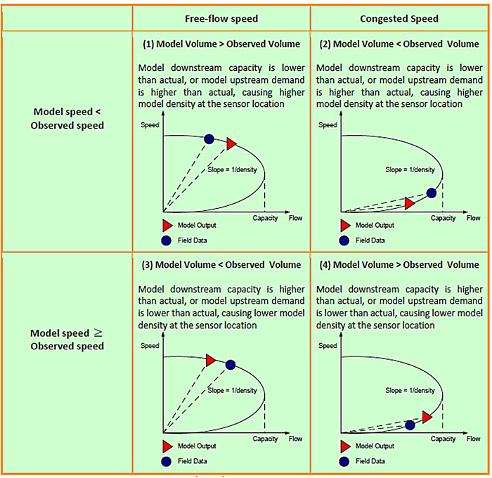
Source: DTA Primer.
8.7 Model Validation
It is important that validation data be cleaned and free of inconsistent abnormalities. Frequently, the validation data set consists of data that have not been used for calibration. It is valuable to test the model’s response to a change in the transportation system and not only its ability to reproduce the base-year conditions. If field data exist from a period in time before or after the base-year model, the analysis team can validate the direction and magnitude of the change the model predicts against observed data. Such a comparison can provide confidence to the stakeholders of the model’s predictive capabilities. If the model’s response is not satisfactory, the base-year model can be recalibrated with a new set of parameters that more accurately predict the non-base-year conditions while maintaining the fit of the original base year model. This subsequent validated model is then utilized for analysis.
In some transportation modeling applications it can be challenging to obtain one good data set for model calibration let alone obtain a second dataset for model validation. As the availability of data improves through technology, the ability to conduct a robust model validation will become less costly. Conducting validation of models will help increase the confidence in model results.
8.8 Model Calibration Checklist
A checklist has been developed describing the model calibration process discussed in this chapter. This checklist may be altered as needed by agencies as specific calibration requirements are developed.
❑ Prepare base model (see Chapter 6).
❑ Error check base model (see Chapter 7).
❑ Review and update calibration objectives: It is likely that time has passed since the project was scoped and the objectives of calibration were developed. Take time to review the objectives prior to any calibration activities. The objectives should be guiding principles and provide direction as to the priority of calibration. Ensure that over the course of the project there has not been a change in focus or direction, and update the calibration objectives as needed.
- Where is the primary area of concern within the model for calibration?
- What model performance measures are most important for calibration?
- What are the statistical criteria for calibration acceptance?
❑ Assemble performance measures used for calibration: The performance measures used for calibration have been identified during the identification of calibration objectives. In the data collection part of the study, the data for calibration have been collected and documented.
- Assemble calibration data into a format that can make it efficiently comparable to model outputs.
- Prepare model output formats that are readily reproduced and will facilitate the iterative process of calibration.
❑ Establish model calibration criteria.
❑ Stress Test Model: (See Chapter 7 for guidance) A pre-calibration activity that occurs after the base model has been constructed and errors and mistakes have been eliminated in the testing of model sensitivities.
❑ Develop Calibration Strategy:
- Review software vendors’ recommended approach.
- Prepare stopping criteria for DUE.
- Develop an approach and sequence for adjusting model parameters.
❑ Conduct Calibration Runs:
- Run model and compare results.
- Implement calibration strategy.
- Develop calibration statistics.
❑ Report Calibration Results.
❑ Validation:
- Prepare second model data set.
- Prepare second set of calibration data.
- Run calibrated model with new data set.
- Compare model results and field performance data.