Traffic Analysis Toolbox Volume XIV: Guidebook on the Utilization of Dynamic Traffic Assignment in Modeling
9.0 Alternatives Analysis
9.1 Short-Term versus Long-Term Impacts
DTA can be used to analyze both short-term and long-term impacts of an alternative of interest. A short-term impact can temporarily motivate tripmakers to adjust their travel choices, such as departure time, route, etc. If this travel choice change is a temporary reaction to the stimulus and the tripmakers soon revert back to their original habitual travel choice, then this temporary effect is considered a short-term impact. On the other hand, if the stimulus is persistent over time or is of high magnitude that generates fundamental and long-term behavior change, the effect is considered a long-term impact.
Short-Term Impact Analysis – Non-Equilibrium-Based DTA
It is difficult to define the temporal span of what is “short-term” or “long-term” because this definition varies by person or situation. This guidebook suggests that the short-term analysis aims to depict the congestion immediately after the start of the stimulus up to a certain period thereafter. During this period, tripmakers traveling on their habitual routes in the impact area may or may not anticipate severe congestion. A portion of the tripmakers may try various means to assess the situation (e.g., congestion experience or information from media sources or other en-route information) and decide on the best course of action, which could include changing departure time, route, or mode choice.
From a modeling standpoint, the short-term impact could be captured by having tripmakers initially follow their habitual (DUE) routes if their departure time is prior to the start of the incident, until they begin to receive external stimuli that motivate their possible diversion from their habitual routes. If they depart during the incident period, then their choice may be influenced by stimuli such as traffic information. The non-equilibrium-based DTA modeling approach may be suitable in this modeling context.
Modeling short-term impacts using a non-equilibrium DTA approach mostly involves a one-pass run of simulation. When tripmakers start their trip with the habitual paths typically obtained from the DUE baseline case, they exercise various diversion decisions when faced with unexpected congestion or new traffic information. The pre-trip/en route diversion rules will determine where, when, and why a trip-maker diverts. Generally, the reaction behavior could be modeled in pre-trip or en-route simulations as described below.
- Pre-trip. Tripmakers may choose to change their routes should they be informed that their habitual routes are impacted by an unexpected incident; otherwise, tripmakers may continue with their habitual routes.
- En route. Tripmakers may choose to divert (when possible) taking into account availability of diversion points should they experience unexpected delay or are informed about extraordinary driving conditions by roadside devices such as dynamic message signs (DMS) or in-vehicle telematics such as radio, GPS, smartphone, or other mobile computing devices.
The number and logic of diversion rules could vary by decision context. How frequently a trip-maker is exposed to such decision contexts, and how frequently a trip-maker is making such a decision, continues to be an active research area. The actual implementation of these rules could vary across different software model systems.
Long-Term Impact Analysis – Equilibrium-Based DTA
In the event that the stimuli are temporally persistent, some impacted tripmakers may seek and settle on other good routes for future use. The outcome of such a learning and adaption process is new habitual route choice behavior. The long-term impact analysis is aimed at understanding the extent of the trip-maker deviating from his/her prior habitual route/departure time to another possible route/departure time and how such a decision may impact other roadways. The equilibrium-based DTA approach appears to be the most suitable for modeling such long-term impacts.
Multiple Trip-Maker Classes
Accurately depicting heterogeneous travel choice behavior continues to be one of the greatest challenges in the development and research of traffic analysis models. A simulation-based DTA approach can resolve this challenge by being flexible to simultaneously simulate tripmakers stratified with different route choice objectives and/or information access. This is called the “multiple trip-maker class” (MTC) concept in literature. The MTC concept allows the model analysis team to capture the impacts/benefits of various ITS strategies by specifying the market share of tripmakers with different route choice objectives. The actual utilization of such a feature could vary between software implementations.
9.2 Random Variation
Microsimulation guidelines recommend that multiple model runs with different random number seeds are necessary to produce statistically significant distributions of model outputs. Running multiple runs takes into consideration that microscopic models involve a wide range of random processes throughout the simulation. There is ongoing research regarding whether the same process should be applied to simulation-based DTA models, but doing so is technically feasible and sound.
Two issues need to be considered when addressing random variation. First, if a mesoscopic traffic simulation approach is used, it is theoretically known that random variation is smaller than that in a microscopic model if the O-D attributes of the simulated population remain unchanged across scenarios. On the other hand, if the O-D attributes also vary across compared scenarios, then the random variations will be greatly increased. Under the varying O-D attribute condition, multiple model runs may be needed to provide statistically significant results. The number of model runs and the time it takes to run the model set should be considered in the scope. For a smaller model this may not be significant effort, but in larger models this could take longer and impact the schedule and resources.
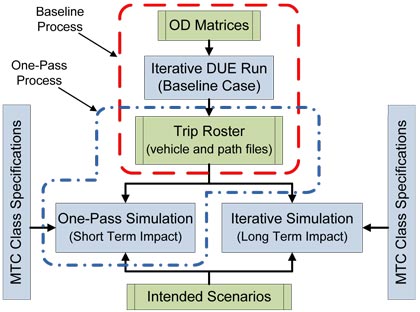
Another approach is to generate a vehicle roster from the baseline case and keep the same identical population/trips across different scenarios. The purpose is to keep trip-maker attributes (e.g., departure time and O-D pair) unchanged across scenarios, thereby eliminating the randomness introduced by O-D variations. The possible drawback of this strategy is that the analysis is based on one set of demands and not on a range of demand variations. The general procedure to ensuring demand/trip consistency, as shown in Figure 9.1, entails the following steps:
- Start with the baseline case by using time-dependent O-D trip matrices or a trip-maker trip roster produced by an external source as the trip-maker generation mode and run the DTA model to DUE.
- At the end of the DUE run of the baseline case, regardless of the demand generation mode (O-D or trip-maker trip roster), the DTA model will produce output containing attributes of each simulated trip-maker and the last-updated trip-maker path from the baseline case.
9.3 Warm Start versus Cold Start
Having each vehicle start with a habitual path from the base case is called a “warm start,” which typically converges faster and produces more consistent results than a “cold-start” model run. A cold start means starting the DTA model without using previously converged DUE paths.
A warm start would be appropriate if the same trip roster is used from the baseline case to ensure that identical trips are being modeled and compared. In this case the output of each trip-maker’s last-updated path from the baseline case is used as the initial path in the compared scenario case. If the scenario involves a significant demand change from the base case then the warm start is not an option.
Figure 9.1 Baseline and Scenario Modeling Framework
Source: University of Arizona.
9.4 Stand-Alone DTA Analysis versus Integrating with a Demand Model
A DTA model can be used as a stand-alone model system or be integrated with a demand forecasting model. If a DTA model assumes that the demand is an exogenously given model input, then the model is to address the route choice decision only. One common concern is how other travel choices may be affected by the scenario of interest (e.g., departure-time choice or mode choice), and addressing this issue may require integration with a demand forecasting model.
Stand-Alone
When using a DTA model as a stand-alone model, the choice dimension being addressed is mostly route choice, unless the DTA model is either integrated with other demand forecasting capabilities or designed to simultaneously model multiple choice dimensions. When performing scenario comparisons, it is critical to keep the population/trips identical across different scenarios in order to ensure that departure times, O-Ds, and attributes remain unchanged. If the alternatives of interest are modeled using vehicles with different trip O-D pairs or attributes, then randomness may be introduced, hindering the ability of the analysis to depict the true impact of the scenario of interest. Although different DTA models may have different ways of implementing such characteristics, it is critical for an analysis team to ensure consistency across compared scenarios.
Feedback Framework
The need for a feedback between DTA and travel demand model varies by project purpose and analysis context and applications. In general, if the scenario of interest is deemed to trigger multidimensional travel choice adjustments, such as departure time and/or mode choice, then the analysis should consider an appropriate feedback framework and procedure to depict such choices.
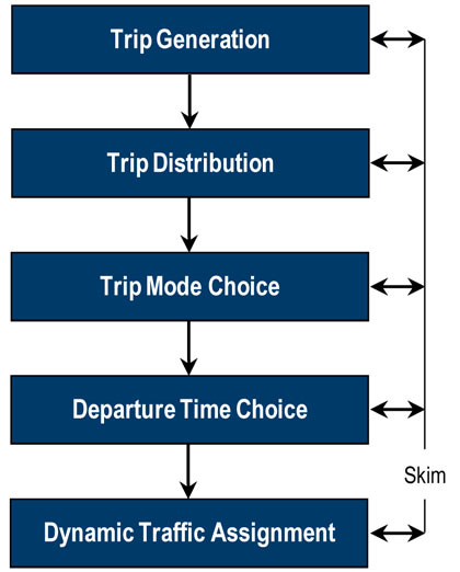
The feedback process could be generally supported by either a trip-based or activity-based model framework. The trip-based model framework, as shown in Figure 9.2, takes the so-called “skim” data (zone-to-zone travel times) and feeds these back to various prior steps to re-estimate trip generation, distribution, mode share, and/or departure time choice.
Figure 9.2 DTA Feedback in a Trip-Based Travel Forecasting Framework
Source: University of Arizona.
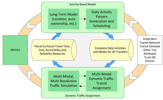
The main feedback mechanism from DTA to an activity-based model (ABM) is the so-called skim matrices, which are the zone-to-zone (or parcel-to-parcel or location-to-location) travel times informed by the traffic simulation model. The change of travel time due to the scenario of interest could trigger the adjustment of different travel decisions. The concept of the SHRP 2 C10 feedback framework is illustrated in Figure 9.3.
Figure 9.3 Feedback Project Modeling Framework
Source: Cambridge Systematics and University of Arizona.
9.5 Interpreting Model Outputs
Resources for interpreting results include:
Simulation-based DTA models generally provide MOEs at vehicle/person, link, path, corridor, and network levels.
Vehicle/Person Level
When the same vehicle roster is utilized in all compared scenarios, vehicles with the same ID in different scenarios can meaningfully be compared. For example, in the baseline case, all the vehicles passing through a work zone link can be tagged, and then the chosen routes of these vehicles can be compared before and after the work zone.
Link Level
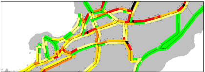
In the link-level comparison, individual route choices and travel interact to form aggregated time-varying MOEs at each link of the network. The diversion in the work zone example also could be depicted and understood by comparing the volume/speed difference before and after the work zone to infer the total diversion around the work zone impact area. Figures 9.4 and 9.5 are examples of model outputs utilizing link-level analysis. In Figure 9.4 the red bands indicate where traffic volumes have decreased while the green bands indicate where traffic has increased. The thickness of the bands is an indication of the magnitude of the change in traffic. Figure 9.5 illustrates different levels of congestion by roadway link..
Figure 9.4 Link Volume Difference between Two Different Sets of Model Results
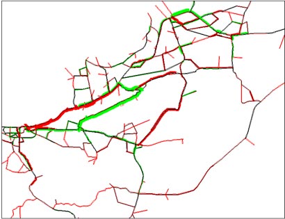
Source: University of Arizona.
Figure 9.5 Speed/Density Plot for Links
Source: University of Arizona.
Path Level
Another way of reviewing the results is as follows: for a given O-D pair and departure time, show the set of used paths and their respective travel flow. The path sets and assigned flows for the given O-D pair will change by time. Visualizing the path set and flow change is a powerful way of depicting the model outputs.
Corridor Level (Heat Diagram)
A common approach to showing the spatial and temporal extent of congestion is the space-time diagram (i.e., speed contour diagram or heat diagram). Figure 9.6 provides a sample speed contour diagram. The diagram shows the speeds occurring in the freeway, where green indicates speeds greater than 65 mph, while red indicates speeds less than 25 mph. Time is represented from left to right while the distance is from top to bottom.
Network Level
The network-level results can be displayed and analyzed textually or graphically. Most DTA software models generate overall statistics reports for the analyzed scenarios, but such network-wide statistics may be misleading if not interpreted carefully. For example, the impact of a work zone represented as a percent travel-time increase could vary depending on the extent of the area chosen as the basis of comparison. As a result, it is important to properly define the impact area for scenario comparison.
Graphical or animation representation of the simulation results for the entire region also will reveal local areas of congestion or critical spots. This information is useful for visual inspection and for understanding the characteristics, congestion. and/or impact of the scenario of interest. Figure 9.7 shows an example of network-wide animation of traffic dynamics.
Figure 9.6 Speed Contour Diagram for Corridor-Level Analysis
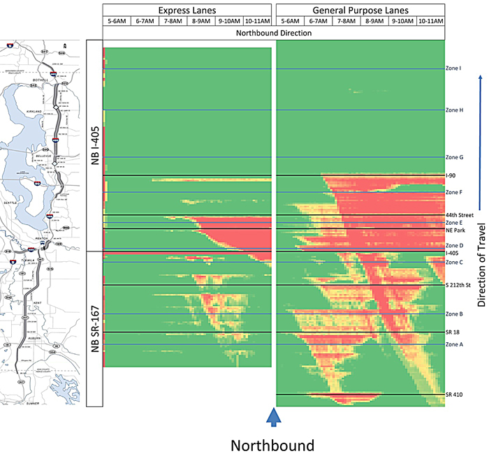
Source: Cambridge Systematics, Inc.
Figure 9.7 Network-Wide Animation of Traffic Dynamics
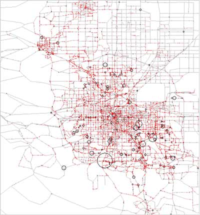
Source: University of Arizona.