Traffic Analysis Toolbox Volume XIV: Guidebook on the Utilization of Dynamic Traffic Assignment in Modeling

7.0 Error and Model Validity Checking

The purpose of error checking (identifying mistakes) and validity checking (model diagnostic runs) is to improve the quality of the models prior to calibration and alternatives analysis. Some of the biggest sources of rework and difficulty in calibration occur when network coding errors have not been identified and addressed. In these cases, instead of comparing the simulation results to field data during calibration, the analysis team is either uncovering mistakes in network coding, or worse, attempting to match field data with an error-prone network. A thorough quality control process should be in place to examine and remedy such coding issues. A good quality control process involves a systematic checking of a model by a knowledgeable person who is independent of the network developer.

In addition to error checking the model files, it is important to conduct a series of diagnostic model runs to verify that the model reasonably represents travel conditions and behaviors observed in the field. This chapter discusses different types of diagnostic runs that are designed to identify issues in the model, prior to conducting the model calibration process. Often these diagnostics tests are considered to be part of calibration. This guidebook recommends tackling this step prior to the start of calibration to allow the focus of the calibration to be on adjusting the model parameters to match field results. Figure 7.1 presents the steps involved in the error and model validity checking process. Descriptions of each of these steps are provided in the following sections.

Figure 7.1 Error and Model Validity Checking Process

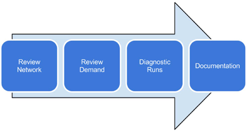
Source: Cambridge Systematics and University of Arizona.

7.1 Network Review

Once the network has been converted to the appropriate format for the DTA model, it is best to further examine the properties and attributes of the network, including links, link-to-link connectivity (i.e., nodes or link connectors), traffic control properties, zone and demand data, and any other fields of information regarding the created network.

Network Connectivity

Common examples of network connectivity issues to be considered are as follows:

• Missing connections (e.g., a ramp interchange is missing);
• Link directionality (e.g., links coded opposite of the intended direction);
• Lane connectivity:
  • Moving from a link with more lanes to a link with fewer lanes,
  • Moving from a link with fewer lanes to a link with more lanes, and
• When GIS files are assembled from different sources to create one cohesive file for model development, the blending of the files may contain errors.

Link Speed Limits

A network converted from a planning model will most likely not contain existing speed limit information; however, estimated free-flow speeds from the model would most likely be available. The analysis team may choose to use this information, but examining the variance of assumed speed limits is wise.

Intersection Geometry

The goals of checking the intersection geometry are to ensure that the connectivity of intersection geometry is correct for each intersection approach and to determine that the geometry is correctly represented. The attributes that should be rectified if not correct include the following:

• Link connectivity;
• Lane connectivity;
• Traffic control;
• U-turn restrictions;
• Turn/lane prohibitions; and
• Turn bay lengths.

The list of link attributes illustrated in Figure 7.2 serves as an example of factors required to correctly capture intersection geometry.

Figure 7.2 Intersection Approach Geometry Attributes

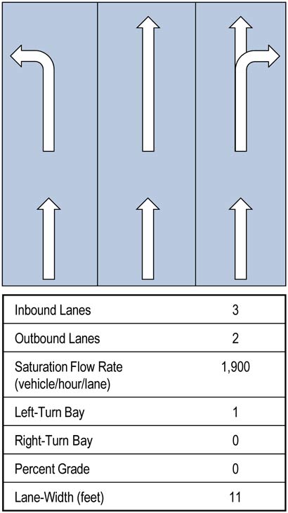
Source: University of Arizona.

Note: Saturation flow rates if required as a model entry are a field measured input.

Traffic Control

Traffic control must be consistent with network connectivity. Mistakes, such as the one demonstrated in Figure 7.3 below, would typically include:

• Skipped signal phasing;
• Signal timings inconsistent with geometry;
• Incorrect cycle lengths, split times, and offsets;
• Missing approaches; and
• Incorrect timing, phasing, offset and coordination.

Figure 7.3 Inconsistency between Connectivity and Traffic Control

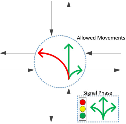
Source: University of Arizona.

Network Paths

Different DTA models may have different ways of generating vehicles entering and exiting the network. Regardless of the model mechanism, each zone in the network should have at least one generating function and one destination function. When checking for network connectivity, the analysis team should be checking that for every zone to zone connection that there are logical and accessible paths for vehicles to take.

Network Coding Checklist

To help improve the quality of work being performed, it is best to have a checklist of all necessary activities. This list should be maintained by both the analysis team and the personnel assigned to quality control. The following is a short example of issues to review in network coding.

• Connectivity:
  • Arterial connectivity at intersection:
    • Correct cross-street connectivity;
    • Turn bays of all approaches;
    • Outbound turn movements; and
    • Number of lanes for each outbound and inbound.
  • Arterial connectivity at non-intersection:
    • Outbound movement directions;
    • Speeds of connecting links;
    • Number of lanes of connecting links; and
    • Freeway ramp connectivity.
  • Ramp turn bays:
    • Allowable turn movements;
    • Link speed;
    • Number of lanes;
    • Outbound connectivity; and
    • Traffic control.
  • Freeway at nonramp connection:
    • Outbound movement directions;
    • Speeds of connecting links; and
    • Number of lanes of connecting links.
• Traffic Control:
  • Correct traffic control at node:
    • Movements are coded for each phase;
    • Phases correspond to correct turn movements;
    • Actuated settings and detectors;
    • Cycle length, green time, amber time, all red time; and
    • If two-way stop sign or yield sign, the major/minor approaches.
  • Network Paths and Connectivity:
    • Each TAZ has at least one generator and one exiting mechanism;
    • Correct downstream connectivity to complete vehicle trip; and
    • Appropriate network functional type.

7.2 Review Demand

The travel demand inputs must also be validated before model calibration. One of the most common difficulties arises in disaggregating the demand from existing peak-period O-D matrices to time-dependent demand matrices at a finer temporal granularity (e.g., 15-minutes). Generally, it is not advisable to take a single 24-hour O-D matrix and apply the diurnal distribution factor to produce the time-dependent O-D matrices. In the single 24-hour O-D matrix, the trip directionality information for the AM and PM periods are aggregated. If time-of-day O-D matrices (e.g., AM peak, mid-day, PM peak) are available, then the trip directionality is inherently preserved in each matrix, and each time-of-day matrix can be directly disaggregated into finer resolution matrices.

Care also needs to be taken in estimating the diurnal distribution of O-D matrices. If vehicle departure associated with an origin is derived from survey data, such as a daily travel survey, then the diurnal factor can be directly applied. On the other hand, if such a distribution is derived from traffic data, then one must consider the time lag needed for traveling from the origin to the data collection point, and the diurnal distribution must be temporally adjusted to account for the time lag.

7.3 Model Validity Checking

Diagnostic model runs help locate and remedy potential coding errors in the network before the start of calibration. Often modelers will find coding errors in the network in the calibration phase, which adds delays to the schedule. An adequate amount of time should be allocated to this stage of diagnostics prior to calibration. The diagnostics stage will require several runs of the model – not for the purpose of producing useful simulation results, but simply for identifying trouble spots in the network.

There are two types of diagnostics: single-run testing and iterative-run stress testing.

Single-Run Testing

Simulation, when used as a diagnostics tool, is unforgiving when finding errors in the network coding. Such instances may include the following:

• Incorrect/incomplete turn movements at an intersection;
• Incorrect signal phase movements at an intersection;
• Lack of connectivity to/from a node or link;
• “Floating” nodes/links;
• Reverse-direction links; and
• Hidden/stacked nodes and links found to be duplicates.

Some errors may come from the conversion process, and some other errors may come from the source of the network. It is best practice to maintain a list of errors to report back to the maintainers of the source network. (Documentation is discussed later in this chapter).

Network Loading

The single-run test can help determine whether vehicles exit the network based on the initial travel routes assigned by the simulation. The demand used for single-run testing can be a short period of demand, such as a fraction of a peak period of demand. Running a portion of demand reduces the computational time for testing and helps find potential coding errors in the network much more quickly. Multiple model runs may be required to identify and fix different coding errors in the network. While executing multiple runs of the model, the analysis team should incrementally increase the demand to 100 percent. At this point, most (if not all) links, approaches, and paths will have been traveled and most obvious coding errors will have been identified.

Testers should also examine network loading locations where vehicles enter the network. Entry queue volumes should be examined for excess queuing and unreasonable delay. Depending on the method of vehicle generation, attention should be paid to whether enough capacity is available for vehicles to enter the network. Possible remedies include, but are not limited to:

• Creating multiple entries for a single origin;
• Increasing the entry capacity; and
• Review if temporal demand/entry volumes are correct

Emptying the Network of All Vehicles

In this test, the important aspect on which to focus is whether the vehicle has completed its trip. This will accomplish the task of determining whether there is a problem with connectivity and false prohibition of movements in the network. If connectivity is incorrect (e.g., the downstream node of a traveler’s starting link is not connected to the network), then the vehicle has no possible way of reaching its destination.

In simulation, there are two time periods: the simulation period and the demand generation period. Demand generation for this testing purpose can be a short period (e.g., a peak-hour of demand). The simulation period for this testing should be a much longer time period. This allows all generated travelers to exit the network, even those vehicles generated late in the demand generation period. Figure 7.4 illustrates these concepts.

After this simulation has completed, the analyst should review the simulation results via numerical output that indicates the number of vehicles in/out of the network after simulation or by reviewing graphical output via animation of simulation results to determine if vehicles are “stuck” somewhere in the network.

Figure 7.4 Cumulative Curves Demonstrating Network Emptying

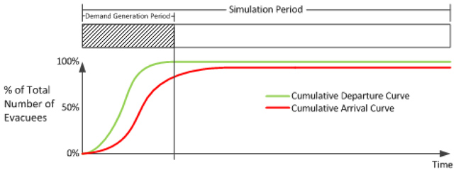
Source: University of Arizona.

Locations of Unreasonable Traffic Flow

When all vehicles have been emptied from the network, the next step is to look into locations in the network that are unreasonable. Simulation results demonstrating long, consistent periods of congestion that do not recover until the end of simulation are indicators of unreasonable results, which include the following:

• Low speed;
• High density;
• Low flow rates;
• Prolonged queuing; and
• Unintuitive used/unused routes.

Errors in link and node/connector attributes are typically identified in these tests.

Stress Testing – Iterative Assignment

Once the single-run testing is completed, the next step is to begin performing stress tests on the network, which essentially means bringing the network to run at full demand. Similar to what was performed with the initial testing, it is best to start off with a lower amount of demand. This means reducing the demand being used by some overall factor that will allow for quicker model runs. The demand should be incrementally increased as any issues are addressed. As stress to the network increases, the confidence in the network conditions grows before undertaking calibration.

Examining the results of a simulation run should include identifying locations that are severely congested and/or that never seem to fully recover. A good test is to trace downstream of these routes and look for the following:

• Limitations to connectivity;
• Incorrect lane count;
• Inappropriate destination locations for exiting trips;
• The appearance of known bottlenecks (may not be correct in intensity but the locations should begin to appear); and
• Incorrect correspondence between demand and the network.

Results from Iterative Assignment

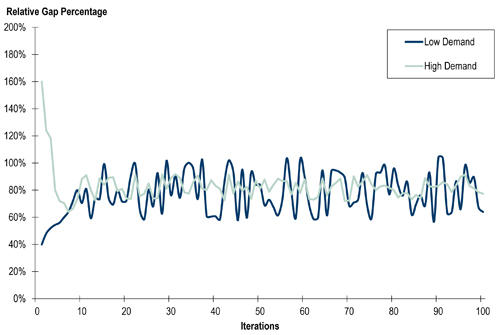
It is important to keep an eye on the numerical results generated by iterative assignment runs: looking at the numerical output summarizing the results of network convergence and stability tell how well the network is running as a whole. The DTA feature within the modeling software must be enabled while conducting these runs. With each iteration, it is important to track the progress (rate of improvement to a “converged” run). A convergence chart should be prepared and used frequently throughout the modeling process. Figure 7.5 illustrates a convergence chart where the model was not approaching convergence. In this example the stress test would be indicating that there are significant issues in the model and the analysis team should go back through the network checklist to confirm if there are any items that were overlooked.

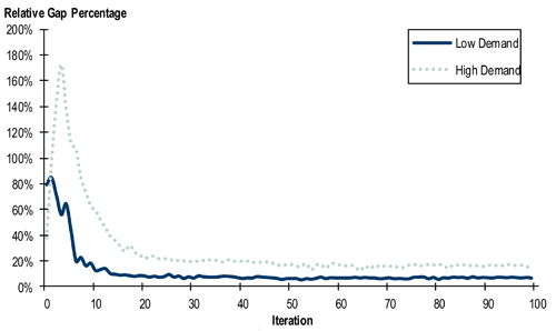
Figure 7.6 is an illustration of the same model shown in Figure 7.5, but with convergence moving in the right direction.

Another aspect to consider in regard to convergence is the stability of the convergence rate. Stability means that convergence has improved steadily over iterations, and at the end of the simulation the change in convergence from iteration to iteration “plateaus.” Other useful metrics to monitor are average travel time, average speeds, average stop time, and average trip distance.

Path Assignment

Another important aspect of running the models to equilibrium is the feasibility of the paths assigned. It is important to understand the core methodology of the DTA tool, especially how paths are determined and assigned. It should be intuitive to recognize paths that are not feasible – for example, paths that are circuitous or far reaching and out of the way. In many cases, these result from local connectivity issues that force path assignment to use what would seem to be the most intuitive paths. In other cases, it may be due to the attributes of the assignment model or other incorrect inputs that require adjustment.

Figure 7.5 Convergence Example: Model not Approaching Convergence

Source: University of Arizona.

Figure 7.6 Convergence Example: Model Approaching Convergence

Source: University of Arizona.

The analysis team also should look for paths that seem to be oversaturated when they should not be according to the existing conditions observed. For example if there is an existing HOV or managed lane that operates at free flow in the field but the model testing has the lanes oversaturated, the DTA model’s method of restricting vehicle classes (HOV, toll, managed lanes) may be incorrectly used or coding could be missing that was supposed to restrict the vehicle classes.

7.4 Documentation

A checklist should be maintained throughout error and validity checking; this can serve as documentation for the technical report. Rather than attempting to remember everything that was performed in the diagnostics phase of the project, analysis teams should continuously report documentation throughout the diagnostics. Also, any errors found in the source model network(s) should be reported back to the originator(s) of the model(s).

Documentation can be as simple as maintaining an Excel sheet logging changes and dating progress or a printed log of changes and dates. Elements to be recorded in the documentation phase include the following:

• Personnel working on network:
  • Date and time of personnel working; and
  • A summary of work being performed (e.g., links, node, freeway, arterial, or other area of focus).
• Individual changes to the network such as:
  • Connectivity correction;
  • Attribute update to link or node;
  • Addition/deletion of link or node; and
  • Identifier of element changed/edited such as link ID or node ID.