Traffic Analysis Toolbox Volume XIV: Guidebook on the Utilization of Dynamic Traffic Assignment in Modeling

6.0 Base Model Development

There are two main components to base model development:

1. Supply. As represented by the transportation network; and
2. Demand. As represented by the trips that travel on the network.

6.1 Development of Transportation Network

DTA models are more data-intensive and less error-tolerant than static models. Often the DTA analysis team works with network data that are as detailed as the data required for microsimulation modeling, but cover an entire region instead of a facility. DTA models, like microsimulation models, are sensitive to the physical characteristics of the network and the presence of signal controls. Erroneous data on a single link or signal with high-traffic volume can significantly influence travel patterns on the network. For this reason, the DTA analysis team should create a network that resembles the physical network as closely as possible.

Depending on the simulation component of the DTA traffic software package, the data required for the network may be similar to either a planning model or a microsimulation model. Often, the analysis team starts with the network from the regional planning model and then adds more detail as needed. Alternatively, one can start from scratch by using public or private datasets, which often contain more roadway links compared to a planning network. The advantages and disadvantages of each approach depend on the data available, coverage, quality, and restrictions.

Link Characteristics

The most important macroscopic link characteristics of a DTA model are the number of lanes, speed, and capacity. Those can be transferred to a DTA model from the regional demand model depending on the compatibility of the data inputs between the two models. Speeds may be set equal to free flow speeds or the posted speed limits depending on the software package definitions. Special attention should be focused on the link capacities, which in planning models are factored down from the Highway Capacity Manual (HCM) theoretical values to account for vehicle interactions such as weaving and the operation of signals and stop signs.

In contrast, DTA models that use either mesoscopic or microscopic flow models do not use capacity as a direct input. Capacities are an outcome of the vehicle interactions, which are affected by link settings such as free flow speed, saturation flow rates, traffic control, and other driver behavior settings. Capacities in these models, when properly applied, are close to the theoretical values of uninterrupted HCM capacity. (For arterials it is about 1,900 vehicles per hour per lane (vphpl) and for freeways it generally exceeds 2,000 vphpl).

DTA models in mesoscopic and microscopic flow models often have additional link characteristics such as vehicle density, driver response time, and look-ahead parameters for lane changing. These parameters are dictated by the simulation methodology and the capabilities of each software package. In order to calibrate this type of model, these parameters are adjusted to reflect observed operations.

Level of Detail

The model network needs to faithfully resemble the physical roadway network. It is important that all the important intersections and roadway links of the study area are imported to the model. If links and intersections are omitted they should generally belong to a roadway functional class that is at least one level down from the roadway class of the links on which the MOEs are collected. For example, if the flow and speed of arterials are to be investigated, the analysis team should make sure to enter collector streets and all their intersections with the arterials. Local streets that provide access to adjacent properties and do not carry through traffic can be omitted and substituted with zone connectors.

As noted, the planning model is a good starting point, but it may not have the level of network detail that is required for a DTA model. For example, in a planning network the number and placement of intersections on a major arterial does not have an impact on the speed of the arterial. In contrast, if an intersection is omitted from a DTA model, vehicles will travel with the prevailing speed and will not stop or wait for a green light or stop sign. To ensure that modeled travel times are not faster than they should be, all critical intersections meeting the functional classification criteria mentioned above should be entered in the model.

Pocket turn lanes, which are generally omitted from planning models, are another example of network detail that cannot be neglected in a DTA model. If a pocket lane is omitted, turning vehicles will delay through-moving vehicles until they find a sufficient gap in the opposing traffic stream to turn. Intersection movement capacity and the resulting delay influences both the simulation times and the routing decisions and cannot be properly estimated unless turning bays and intersection configuration are entered accurately in the DTA model. Aside from pocket lanes, the analysis team should reconsider links smaller than a vehicle’s length, code merge and diverge sections at a junction, and remove centroid connectors connected to intersections and connect them at midblock locations.

Like microsimulation models, some DTA models require the analysis team to explicitly define the lane connectivity at each intersection. Defining the lane connectivity involves determining the movements that use a particular lane (e.g., right turn and through movements for the rightmost lane). Unlike corridor microsimulation models, regional planning models are usually not concerned with intersection geometry and movement capacities.

All simulation-based DTA models, even those that do not allow the user to explicitly define lane connectivity, distinguish between different movement types to calculate delay. Left-turning vehicles facing a signal or opposing traffic may encounter significantly more delay than through or right-turning vehicles. DTA models keep a record of the delay encountered by each vehicle and movement and use this information for path building. This is another difference from the majority of static models, which frequently define delay only at the link level assuming that all movements experience the same delay. When using DTA models that internally define the permissible movements on each lane of an intersection, the analysis team should have an understanding of the internal rules that are applied in the model.

Traffic Control Information

Traffic control information includes information about stop signs, yield signs, lane controls, and traffic signals. Traffic signal data include signal phasing, signal timings, coordination parameters, actuated control settings, and other parameters. Traffic control information can vary from project to project, but it does represent a substantial amount of information that must be accurately entered for the models to operate correctly. Depending on the capabilities of the software, the types of signals a DTA model may simulate include the following:

• Pretimed signals, in which both phase timing and phase sequencing are predefined and do not change during the signal’s operation;
• Single-ring actuated signals, in which the phase sequencing and the movements that comprise each phase are predetermined, but the phase timing varies based on vehicle presence during operation;
• Dual-ring actuated signals, in which both the timing of each phase and the movements in operation vary based on conditions on the ground; and
• Dual-ring actuated coordinated signals, in which the timing and sequencing may change as above, but the cycle length remains constant allowing for signal coordination.

Traffic signal data can be found in various data formats, including relational databases, Excel, PDF, and proprietary data formats that signal optimization software use. Due to the differences in the operational and hardware characteristics of the traffic controllers in the field, a single standard format for storing signal data has not been widely adopted. Instead, many agencies have defined their own custom-built format that is often incompatible with the DTA software and for which a preexisting importer does not exist. As a result, and for a large modeling region involving more than one agency or city, information may come from disparate data sources containing descriptive data that are not easy to associate with the node-link-movement structure of a DTA network.

When signal optimization software have been used to optimize signalized corridors or small areas, the analysis team may be able to use a software importer to transfer the data from the signal optimization file(s) into the DTA model. If the signal optimization software network and DTA network are incompatible with each other, the analysis team will have to develop equivalency protocols before importing signal timing data.

Importing signal data from agency traffic signal controller databases into a DTA model will be difficult if the database format and model input format are not compatible. Creating an equivalency profile or script application to automate the conversion of data is worthwhile if the model includes a large number of intersections.

Time-Dependent Network Properties

DTA models allow for testing the effects of changes that may occur in the course of the modeled period. The types of network properties that can vary by time include the following:

• Traffic signal properties can vary by time of day.
• Network events that can alter the network connectivity or movement characteristics, such as:
  • Incidents;
  • Work zones;
  • Variable speed limits; and
  • Reversible or peak-period HOV lanes.

Fidelity

The types of analyses for which the model will be used determine the level of detail required. A rule of thumb is to code in transportation facilities that are one functional class level below the level of interest for the study. One highway network may be used to represent the entire day, but it may be desirable to have networks for different periods of the day that include varying and or operational strategies, such as reversible lanes or peak-period HOV lanes. Multiple period networks representing the strategies being evaluated can be stored in a single master network file that can be activated and deactivated as needed.

Availability of Network Data

Digital street files are available from the Census Bureau (TIGER/Line Files), local agencies (e.g., GIS departments), and commercial vendors. Selecting the links for the coded highway network requires the official functional classification of the roadways within the region, the average traffic volumes, street capacities, TAZ boundaries, and a general knowledge of the area. Other sources for network development include the following:

• FHWA National Highway Planning Network;
• Highway Performance Monitoring System (HPMS);
• Freight Analysis Framework Version 3 (FAF3) Highway Network;
• NAVTEQ Data;
• National Transportation Atlas Database; and
• Various state and metropolitan planning organization (MPO) transportation networks.

All of these third-party resources may be useful as starting points for development or update of a model network; however, each source has limitations in terms of cartographic quality, available network attributes, source year and, especially with commercial sources, copyrights, which should be considered when selecting a data source.

Any use and or transfer of data from third-party sources into models will require review and possibly editing to ensure that the data are in fact correct.

Link Data

Once the initial transportation network has been developed, the analysis team must input the physical and operational characteristics of the links into the model. These include:

• Number of lanes;
• Lane width;
• Link length;
• Grade;
• Curvature;
• Pavement conditions (asphalt, gravel, etc.);
• Sight distance;
• Bus stop locations;
• Crosswalks and other pedestrian facilities;
• Bicycle lanes/paths; and
• Other data.

The specific data to be coded for the links will vary according to the DTA software. Many of these attributes are stored in local jurisdictional databases and can be transferred to the highway network links. In the absence of readily available data, the data can be manually collected in the field.

Traffic Operations and Management Data for Links

Traffic operations and management data for links consist of the following:

• Warning data (incidents, lane drops, exits, etc.);
• Regulatory data (speed limits, variable speed limits, HOVs, high-occupancy tolls (HOT), detours, lane channelization, lane use, etc.);
• Guidance information (dynamic message signs and roadside beacons); and
• Surveillance detectors (type and location).

6.2 Development of Origin-Destination Information

Origin and destination information describes the trip making activity that occurs in a transportation network. Ideally, O-D information for base and future-year analyses would be generated by travel demand models as they are well suited to capture travel desires given varying land use. The overall objective is to provide O-;D matrices by vehicle type (e.g., single or high-occupancy vehicle, taxi, and truck) for each time slice during the entire study period that are consistent with ground counts yet sensitive to future-year changes in demand and/or supply.

Methods for Developing O-Ds

The main method for developing information on the spatial pattern of trips within urban areas traditionally has been O-D surveys. When sufficient observations are gathered for statistical reliability, these surveys can be factored up to compute the flows among traffic zones. This information then becomes the basis for the O-D information that is input to the DTA software.

Unfortunately, O-D surveys of a statistically sufficient sample size are expensive and difficult to implement. Traffic data, and in particular, traffic counts are readily available and can be used to synthesize O-D information directly using O-D matrix estimation (ODME) techniques.

Regional travel demand models represent the most comprehensive source of O-D information in that they are calibrated models based on observed data and also have the capability to predict future conditions in a consistent manner.

Travel demand models are designed to capture this trip making information for existing conditions, but more importantly for alternative scenarios including future year conditions. There are two main types of travel demand models that produce O-D information:

1. Four-step models, in which O-D information from conventional trip-based travel demand models is used to produce trip tables; and
2. Activity-/tour-based models, in which O-D information from activity-based models is in the form of trip rosters or trip synthesizers.

The link between travel demand and simulation models is the O-D information, which can be extracted from the regional model to provide demand inputs to the simulation model. By providing a direct link to the regional model, the O-D information is consistent with the regional travel patterns used by the regional model.

Maintaining a connection to changes in regional supply and demand from the travel demand model. Maintaining this connection with the simulation model ensures that regional travel patterns are reflected in the base and future O-Ds, including the following:

• Distribution of travel demands as reflected by the regional model’s destination choice models;
• Mode shares reflective of supply and demand dynamics embedded in the mode choice models within the regional model;
• Incorporation of traffic count data that provide a more realistic representation of the operational characteristics of the existing transportation network;
• Refined models to estimate smaller time increments and to incorporate peak spreading sensitivity; and
• Procedures to pass on the adjusted O-D patterns from the validated base-year matrices to the future O-D matrices.

Figure 6.1 shows an example of the process that was developed for a study in Buffalo, New York. It illustrates the flow of data and highlights the steps and procedures that enable a direct connection between the travel demand model and a simulation model using DTA. The text that follows explains each of these steps.

Figure 6.1 Example Modeling Process Flow Chart

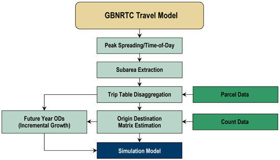
Source: Greater Buffalo Niagara Regional Transportation Council.

Linking Travel Demand Models and DTA

Travel demand models are usually regional in scope as they are primarily used to estimate future conditions over a wide area. Regional models usually have less detailed networks than corridor-level models because the goal of the regional model is to estimate regional travel patterns. The TAZ system that accompanies the regional network also is less detailed and thus not suitable to support detailed traffic analyses. As a result, the O-D matrices that are extracted from the regional model usually cannot be used directly for the DTA model; they need to be disaggregated to a finer level. The granularity is determined by the objective of the transportation analysis.

The starting point is identification of the links within the regional model that represent the extents of the network that will be used for the DTA model. These links form the basis of the subarea model. The base-year subarea model components are then updated to reflect as realistic a representation as possible of the facilities within the subarea corridor. This includes the following:

• Updating the roadway network to ensure accurate representation of the simulated areas, including all ramps and intersections that will be simulated; and,
• Disaggregating the TAZs and the accompanying O-Ds within the simulation model extents to a more refined zonal structure in order to accurately load the traffic.

Figure 6.2 shows an example of a subarea network of the Scajaquada Expressway Corridor in Buffalo, New York (the facilities to be simulated), in the context of the larger regional model network. Figure 6.3 shows an example of smaller subarea TAZs overlaying the larger regional TAZs in the study area in order to more accurately represent trip generators in the subarea network.

Subarea Extraction

Subarea extraction is a common procedure that is embedded in most planning model software packages that enables the user to extract the network and related trip table as defined by the extents of the subarea into new files. These procedures are performed during the assignment phase and produce O-D trip tables for the subarea for each individual time period. These subarea O-Ds form the basis of the seed matrices for the corridor-level demand calibration.

Figure 6.2 Example Subarea Network

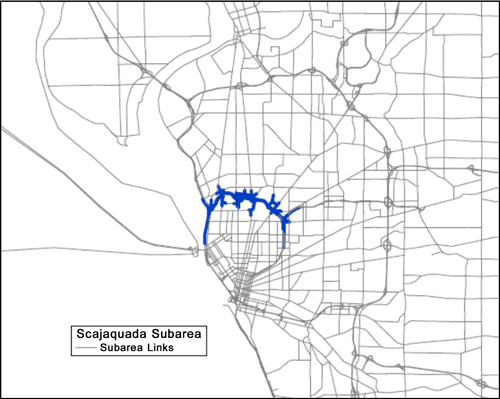
Source: Greater Buffalo Niagara Regional Transportation Council.

Figure 6.3 Example Corridor TAZ Disaggregation

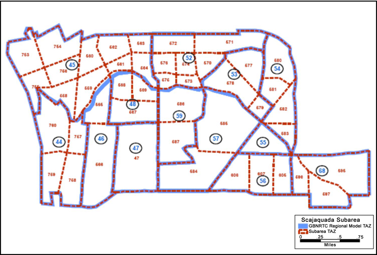
Source: Greater Buffalo Niagara Regional Transportation Council.

Approaches to Disaggregation

There are several approaches that can be used to disaggregate trips from larger regional TAZs to the smaller zones. One simple approach is to distribute the trips (origins and destinations) to the smaller subarea zones based on the ratio of the area of the subarea zone to the larger regional zone. This approach does not take into account where the development is located in the regional zone, nor does it consider what kind of development resides in what part of the zone. It should be taken into account that different land uses have sometimes very different trip generation characteristics.

A better approach is to distribute the trips based on the actual land uses within each of the smaller subarea zones. Using parcel data or other land use data that are defined at the local level, estimates of trip making activity at each of the subarea zones can be made by applying trip rates to the land use from sources such as the Institute of Transportation Engineers (ITE) Trip Generation Manual or by applying the trip rates developed for the regional model. These estimates of trip activity can then be used to redistribute the regional zone-based trips.

The updated disaggregated subarea zonal layer then becomes the TAZ layer for the regional model. New centroids and centroid connectors are added to the network to provide access to/from the new subarea zones and the regional model is rerun with the updated inputs.

Time of Day and Peak Spreading Models

Most traditional regional travel demand models are calibrated and validated to large time periods and are estimated by applying regional factors to every O-D pair based on observations from a travel survey or from observed traffic data. These same regional factors are usually applied to future-year forecasts as well. This approach assumes that the temporal distribution of trips is constant by geography and by time, regardless of the location and temporal extents of congestion. DTA not only requires much smaller time increments in order to simulate traffic operations accurately, but also the level of trip making in any particular time slice is sensitive to the level of congestion at that particular time. Travel demand models employ static methods of assignment and allow traffic volumes to exceed capacity; therefore, it is highly desirable that the method selected for slicing up the O-D information into smaller time intervals is one that considers the level of congestion in the system.

Many of the more sophisticated activity/tour-based models are sensitive to differing levels of congestion and do provide trip (or tour) departure information at smaller time increments. As more agencies develop these types of models, the linkages between the demand-side and the operational models will become more commonplace.

In the absence of sophisticated time-of-day models, there are other methods based on empirical data that can be applied. One such method relies on the fact that there may be a different temporal distribution for every O-D pair that is related to the level of congestion between that O-D pair. For O-D pairs that experience little or no congestion, no peak spreading will occur. For O-D pairs that experience high congestion levels, significant peak spreading will occur and will continue to occur as congestion increases over time. In other words, the level of temporal redistribution is sensitive to changes in demand over time or in response to changes in network supply.

This approach uses estimates of hourly demand and is sensitive to changes in supply and/or demand assuming that the amount of temporal spreading that is likely to occur between any O-D pair is based on the level of congestion that is present along the shortest path between that particular O-D pair. A set of temporal distributions was developed by Margiotta, et al. (Margiotta, R., H. Cohen, and P. DeCorla-Souza, Speed and Delay Prediction Models for Planning Applications, Sixth National Conference on Transportation Planning for Small and Medium-Sized Communities, Spokane, Washington, 1999) that vary based on the level of congestion as measured by the daily volume to hourly capacity ratio (AADT/C). These distributions were developed as a mechanistic way of moving demand from one time period to another as the level of congestion changes. Figure 6.4 shows an example of how the distribution of trips over the entire day might change in response to different levels of congestion.

Figure 6.4 Daily Profile of Trip Departures

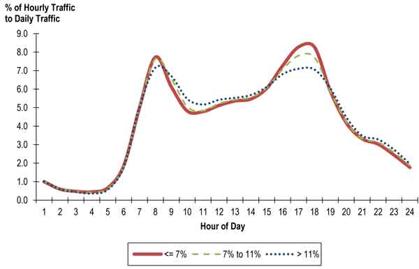
Source: Cambridge Systematics, Inc.

Matrix Estimation and O-D Adjustment Techniques

Before the O-D information can be used reliably to represent base-year conditions, it must be calibrated to observed traffic data. One calibration approach is to further refine the travel demand model itself so that it produces outputs that more closely match observed traffic conditions. Adjustments to the model can be made to achieve this depending on the availability of observed data as well as time and resource constraints. This method can be a valid approach for estimating future year traffic simply by applying the refined travel model and maintaining a direct link between the regional travel model and the DTA model.

Another approach is to adjust the O-D matrices themselves. This can be a manual process whereby the analyst assigns the O-D information to the transportation network and then compares the assignment results to the observed data such as traffic counts. These comparisons form the basis for adjustments to the O-D information in order to get a better fit. The adjusted trip table is then reassigned and the process is repeated until a good fit has been achieved and the O-D information is calibrated. Fortunately, automated processes have been developed to perform this calibration step, which is commonly known as Origin Destination Matrix Estimation (ODME).

Most ODME methods in use today are based on an iterative, bi-level process that switches back and forth between traffic assignment and matrix estimation. The overall objective is to provide O-D matrices by vehicle type (e.g., auto and truck) for each time slice that are consistent with ground counts yet sensitive to future-year changes in demand and/or supply. Implicit within that objective are the following considerations:

• Maintaining consistency with route choice behavior so that predicted traffic flows can be estimated as the result of an assignment process in which a predicted O-D matrix is assigned on the network. Link utilization is flow-dependent, and should be calculated with equilibrium flows.
• Achieving a balance between the need to closely match the target counts and the desire to find a new matrix that is close to the prior matrix, as estimated by the regional travel demand model.

Currently, most of the automated matrix estimation processes are built for use with static assignment models. Static and dynamic assignment methods can produce very different travel paths in the model. As a result, the adjusted O-Dss within the DTA models must be tested to see if path choices are similar enough to produce consistent traffic flows. This can be an iterative process where capacity and delay information from the dynamic models is passed back to the static models and the matrix adjustment process is rerun until a good fit has been achieved. Research efforts are underway to develop matrix estimation techniques that utilize a dynamic approach.

Estimating future year travel using this approach involves an additional step in order to bring together the changes in travel demand as estimated by the travel model with the adjustments to the base year trip matrices that may have been made during calibration. A common approach to achieve this is to calculate the growth component for each traffic analysis zone or each O-D pair and apply that to the calibrated base year demand. This incremental approach does maintain a link between the regional travel model and the DTA model. Care must be exercised using this approach as it is possible for these adjustments to produce negative or counter-intuitive forecasts.