CASE STUDY 5: CHICAGO STREET NETWORK
Project Description
Previous case studies have examined simulation models for before and after construction projects. This case study summarizes an academic validation exercise using extensive before and after data on a complex arterial network signal timing improvement project, compared with micro-simulation projections. The purpose of this study was to investigate key issues in the validation of transportation models and to advance an effort to address them. Many of the issues described are common to models and modelers in all areas of science and engineering.
A test bed was used to provide a mechanism for validating simulation models. This test bed is a microscopic simulator in an application to assess and select signal timing plans on an important street network in Chicago, Illinois.
For the computer simulation model to fulfill its purpose, two crucial questions must be addressed:
- How well does the model reproduce existing field conditions?
- Can the model be trusted to represent reality under new, untried conditions, such as revised signal timing plans?
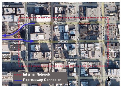
Figure 11: Test Bed Network
The test bed for the study is the network depicted in Figure 11 below. The internal network is defined as Orleans to LaSalle and Ontario to Grand. Traffic in the network flows generally south and east during the morning peak and north and west in the evening peak. This demand pattern is accommodated by a series of high-capacity, one-way arterials such as Ohio (eastbound), Ontario (westbound), Dearborn (northbound) and Clark and Wells (southbound), in addition to LaSalle (northbound and southbound). Traffic generally flows south and east in the morning and north and west in the evening through this signalized intersection network. The question being addressed was to quantify how well simulation, with proper calibration, reproduces the patterns as experienced in reality.
Characteristics and Inputs
Microscopic simulation represents single vehicles entering the road network at random times moving second-by-second according to local interaction rules such as car-following logic, lane changing, response to traffic control devices, and turning at intersections according to prescribed probabilities. The network has 112 1-way links, 30 signalized intersections, and about 38,000 vehicles moving through it per hour. Streets are modeled as directed links with intersections as nodes.
There are a variety of inputs or specifications that must be made, either directly or by default values provided. Signal settings are direct inputs and were singled out as controllable factors since altering these inputs to produce improved traffic flow drives the study. For validation, the signal plan will be the one in the field. For finding optimal fixed-time signal-timing plans, the signal parameters will necessarily be manipulated.
Data Collection
Initial field data for the network were collected on a single day, 7 am to 10 am and 3 pm to 6 pm with the analyses limited to the three one-hour periods, 8 am to 9 am, 4 pm to 5 pm, and 5 pm to 6 pm. This covered the peak periods and a "shoulder" period. Traffic volume data were collected manually and by video recording.
There were very few pedestrians, and they had no discernible effect on traffic. Incidents were not included, but because illegal parking was an endemic condition, the network was coded to account for its effect. Free-flow speed was selected on the basis of posted speed limits. Signal timing plans and bus routes were collected directly in the field.
Analysis and Results
The interest in the model here is its value in assessing and producing good time-of-day signal plans. Comparisons between the field and model results were made through selected evaluation functions to deal with the issues raised.
Evaluation Functions
Stop time (stopped delay) was chosen on approaches to intersections as the primary evaluation function as the typical measure by which intersection level of service (LOS) is evaluated. Other criteria such as throughput, delay, travel time, and queue length are all highly correlated with stop time. Drivers on urban street networks are particularly sensitive to stop time, spurring traffic managers to seek its reduction. In fact, the Highway Capacity Manual's (HCM) selection of stopped delay for LOS designation is meant to reflect the user's perception of the intersection's quality of service.
The quantities for STV (stop time per vehicle) or STVS (stop time for vehicle stopped) for aggregations of approaches (routes or corridors) are very difficult to obtain, requiring the tracking of individual vehicles. By summing over the individual links, a "pseudo stop time" is created for the corridor. This will be close to a real stop time, provided vehicles turning off of or onto the corridor exhibit no difference from those traveling through.
Calibration
Calibration is adjusting input parameters to match model output. Two types of calibration were done in the test bed example. The first addressed the blockage of turns at two intersections and the subsequent gridlock. The network was altered to facilitate the bypass of the blockage without affecting throughput. The second was necessary because of a substantial difference on one link (at the LaSalle/Ontario intersection) between the field and the model stop times. This difference was largely resolved by changing the free flow speed from 30 miles per hour (mph) to 20 mph to be consistent with the observed (from video) speed of vehicles as opposed to the speed limit.
Throughput Comparison
A net change in internal total throughput indicates discrepancies showing less output in the morning and more output in the evening. This is due to the garage effect: vehicles disappear to the parking lots in the morning and reappear from them in the evening; since the morning and evening runs do not span the entire day, there are invariably differences in the counts. The means of 100 replicated model runs are close to the observed counts.
Stop Time Comparisons
The distribution of stop time at each approach shows definite discrepancies at some locations. Examination of video and model animation exposes the key cause: the model does not fully reflect driver behavior. Lane utilization in the model is not consistent with lane utilization in the field. Vehicles joining long queues where they are briefly stopped may not appear in the simulation as having stopped. This accounts for smaller STVS in the field than in the model. The STVS is larger in the model because it counts only vehicles that completely stopped, so the average time per stop is higher However, the key measure of how long truly stopped vehicles are delayed appears to match what is seen in the field quite reasonably.
| Link | Model | Reality |
|---|---|---|
| SB Ohio at LaSalle | 0 | 3 |
| SB LaSalle at Ohio | -11 | -10 |
| NB LaSalle at Ontario | -9 | -5 |
| NB Orleans to Freeway | 13 | 15 |
| NB Orleans at Ontario | 1 | -2 |
A new signal timing plan was put in place in September. Under these new circumstances, predictions were to be made and data collection designed for a day in September expected to be similar to the date of the first data collection in May. The model was run with the May input, except for the updated signal timing. After the data were collected in September, the results were compared on several key links. This showed that throughput and stop time performance (STVS) were reasonably close. However, when the effect of change in demand was checked, it was noted that the model has difficulty dealing with storage of vehicles on short, congested links just downstream of a wide intersection.
| Level of Service | Stopped time per Vehicle STV: Seconds/Vehicle |
|---|---|
| A | STV ≤ 5 |
| B | 5 < STV ≤ 15 |
| C | 15 < STV ≤ 25 |
| D | 25 < STV ≤ 40 |
| E | 40 < STV ≤ 60 |
| F | STV ≥ 60 |
The model differences (Δ = September STVS - May STVS) were compared to the corresponding change in the field values. Even though the model's predictions were not always accurate, the differences are close. This is particularly important for comparing the performance of competing signal plans. A difference of 5 seconds in stop time can be minor but a difference of 15 seconds may be major. One starting point may be a comparison of the field and model-predicted LOS. The 1994 HCM thresholds for LOS were used to be consistent with the use of stopped delay, which was more easily measured.
Spillback
A major difficulty is the model's propensity to turn spillback into gridlock; inadequately modeled driver behavior led to intersection blockage far too frequently. (This was corrected by modifying the network.) The model tended to stop more vehicles than indicated in the field. In reality, drivers coast to a near stop then slowly accelerate through the signal, but the behavior is much more abrupt in the model. This flaw manifested itself in disparate stop rates but did not seriously affect stopped time per vehicle stopped (STVS).
Lane Distribution
It was found that the model was effective but flawed. The model did not accurately model lane distribution of traffic, especially regarding following buses in traffic. Lane selection in reality was much more skewed (drivers refused in general to follow the buses because of the frequent stops) than in the model which showed that most vehicles would follow the buses.
This had some effect but mostly affected the links and not the intersection approaches that would have changed the signal operations.
Conclusions and Recommendations
It was found that the model was effective but flawed, despite properly applied methods and calibration. The process of properly calibrating the simulation is effective and generally applicable when test bed conclusions were derived from the two questions: Does the model mirror reality when properly calibrated for field conditions? Does the model adequately predict traffic performance under revised signal plans?
The approach was to focus on key input parameters, such as external traffic demands, turning proportions at intersections, and effective number of lanes (for example, due to illegal parking), using the model default values for other inputs.
Overall, despite its shortcomings, the model effectively represented field conditions. There is virtually no difference in the estimated levels of service between the field and the model. However, as detailed earlier, there were discrepancies documented with spillback levels, car following and lane distribution, and the "garage effect" skewing the throughput comparison.
The predictability of the model was assessed by applying revised (September) signal plans to the May traffic network. The model estimates of STVS were reasonably close to field estimates and the model LOSs were, for the most part, similar to those observed in the field. More importantly, the model successfully tracks changes in traffic performance over time: on five links for which field data were available, two links exhibited a reduction in STVS, one link an increase, and two had no significant change; the model's predictions were the same.
In summary, a candid assessment of the model is that with careful calibration and tuning, the model output will match field observations and be an effective predictor of operational performance.
Extensions and Guidance
This case study is an excellent example illustrating some potential limitations of simulation and the importance of calibration and validation for practitioners. In this analysis, there were particular shortcomings of the model exposed when comparing its simulation with reality. Some could be overcome with adjustments to the parameters within the model and some were accepted as normal variations.
This points to the need for calibration guidance for users in order to minimize the limitations or flaws in any simulation tool. There were particular steps taken in this study to overcome specific discrepancies. More general guidance could be offered to users to assist their calibration procedures.
Users of simulation models need to fine-tune all inputs that are related to the driving behavior and vehicle characteristics by comparing and adjusting some absolute measures. This procedure for calibration and validation should include:
- Comparing the results from the model with actual field conditions;
- Assessing the applicability of the initial set of parameters, defaults and assumptions;
- Defining acceptable ranges for all parameters for the given analysis characteristics;
- Scrutinizing the results from multiple runs to compare model results with field data;
- Viewing animation against known field operations for any unrealistic conditions;
- Validating new data by comparing results with new field conditions
The flow chart shown in Figure 12 is from "Microscopic Simulation Model Calibration and Validation Handbook October 2006," Byungkyu (Brian) Park and Jongsun Won. This is an excellent tool to guide users through the calibration and validation process necessary for the appropriate use of simulation models.
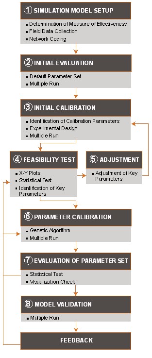
Figure 12: Evaluation Steps
Cross-Cutting Findings
The examples outlined in the case studies provide some insights into common challenges facing transportation agencies today in the arena of microsimulation. While the models sometimes have limitations that might make results differ from actual field conditions, practitioner misapplication or misinterpretation of the results may provide greater variance between model output and field conditions than any limitations built in to the model. If agencies use a defined process for application and interpretation of results and follow the logical steps, many of the common issues can be alleviated. If issues are known, practitioners should be able to understand such limitations and apply the results in a way that ensures sound decisions are made.
| Case | Type of Analysis | Initial Analysis Purpose | Major Challenge Discovered: Comparing Actual to Projections | Major Lesson Learned |
|---|---|---|---|---|
| I-494 & Hwy.7, Minneapolis, MN | Freeway and loop operations analysis | Compare two build (full cloverleaf and partial cloverleaf) and no-build scenarios | Model underestimated flow due to overestimating bottleneck downstream | Compensate for known weaknesses in models, perform sensitivity tests if necessary |
| I-15 Reconstruction, Ogden, UT | Delay comparisons for alternative construction closure scenarios | Compare no-build, conventional build, and design-build construction | Planning model used for analysis failed to estimate acceptably accurate V/C ratios during peak periods | Transportation planning models are limited in providing accurate detailed operational analysis |
| S.R. 826 – Palmetto Expwy. Off-Ramps near Miami, FL | Pre- and post- construction operational LOS for EB off-ramps and auxiliary lane: Microsimulation and HCM | Assist in determining if similar improvements would be warranted for WB direction | Microsimulation accurately projects spillback from increased traffic, and so does not project the isolated improvement from the project | The EB treatment was found to be effective as an isolated treatment; FDOT chose to implement the WB improvement as well for the isolated benefit |
| I-25 & University Blvd. in Denver, CO | Multiple models used to evaluate potential conversion of a cloverleaf interchange to a SPUI | Alternatives analysis comparing cloverleaf upgrade, partial cloverleafs, diamond interchange and SPUI | Simulations projected downstream spillback but alternatives to fix the downstream cause were not developed | A new interchange may operate well in isolation but should usually be viewed in its larger context |
| Traffic Signal Network in Chicago, IL | Signal timing microsimulation projections on complex urban arterial network | Academic validation of before and after signal timing improvement project: How effectively does a well calibrated simulation reproduce reality? | Generally effective, discrepancies in spillback, stopping behavior, lane distribution (e.g. reluctance to follow buses), & “garage effect” for throughput | Demonstrates importance of calibration and validation; all driver behavior and vehicle inputs need fine-tuning |
Freeway widening projects, such as the one in Minnesota, can often shift a bottleneck downstream to another location. Bottlenecks in the roadway system can significantly affect operating conditions. Modeling can help determine the needed expanse for the widening project to avoid major impacts from a bottleneck shifted downstream.
Modelers should be aware that level of service guidelines were designed for use with the Highway Capacity Manual procedures. Metrics such as density and delay that are derived from a microsimulation tool do not provide for direct comparison with such HCM thresholds since they were produced using different procedures. Field measured metrics can be directly compared with HCM LOS thresholds.
Insights into the magnitude and duration of poor operating conditions are important. Often, temporal descriptions of results are needed to help decision makers understand operations. For example, LOS F should be accompanied by the time period over which it occurs, how long it lasts, and if an improvement reduces the metric in question but does not change level of service overall.
Microsimulation projects can require large amounts of data and information. Modelers should build in realistic timeframes that are based on anticipated project-by-project requirements for data collection, processing, and information gathering.
Transportation agency processes often make use of microsimulation models to help determine a particular course of action. More than one "build" alternative may be considered along with the "no build" alternative. Less frequently, microsimulation models are used to predict future performance of the maintenance of traffic alternatives. Expanded use of these tools to predict future construction zone operating conditions can help agencies design a Maintenance of Traffic Plan and help minimize impacts from during construction, as shown in the Utah Case Study.
Microsimulation is not necessarily needed for every potential idea for a project. Agencies should prioritize and identify, based on appropriate information and data, the top alternatives to focus on. Modeling can be useful in supporting investment decisions. The modeling exercise is typically consistent with the scale of the overall project investment.
Tools are available to assist practitioners at the micro, meso, and macro levels (ordered in decreasing levels of detail). For example, a macro level analysis tool is useful in determining future demand for a facility, while a micro level tool allows for additional detail in quantifying impacts at the individual vehicle level. Appropriate timelines and levels of detail should be matched with the appropriate tool.
As shown in the Palmetto Expressway Interchange Case Study, microsimulation can aggregate impacts from multiple improvements. Modelers should determine whether or not they need to understand the benefits and impacts from each individual improvement prior to developing the model. If so, it may be useful to investigate other tools to gain insights into the direct performance of individual improvements. The Denver Case Study was also a good example of how to make use of multiple tools in order to take advantage of the strengths of each.
Prior to model development, data collection plans should be designed to account for unmet demand. Automatic traffic detection equipment typically does not account for demand caused by queuing, but occupancy levels and other measures can be used to determine whether or not saturated conditions may exist. As shown to potentially have occurred in the Denver Case Study, lack of information on unmet demand can significantly affect modeling results.
Queuing is normally adequately accounted for and the effects can be understood using microsimulation. As illustrated in the Denver Case Study, the Highway Capacity Manual procedure is limited in that it does not include the effects of queue spillback at an intersection approach. As shown in the Chicago Case Study, it is important to properly calibrate a simulation model to ensure adequate impacts from queuing are reported and included in the analysis of alternatives.
| Special thanks to Nagui Rouphail of North Carolina State University and Brian Park of the University of Virginia for providing details and insights for use in these comparisons. |