4. Using Toll Tag Readers for Traffic Monitoring

One of the innovative parts of the iFlorida design was the extensive use of toll tag readers to collect vehicle probe data for estimating travel times and identifying incidents. (The system also used a limited number of license plate readers. The focus in this report will be on the toll tag reader network, though many of the observations would apply equally well to a network of license plate readers.) This section of the report describes the iFlorida toll tag travel time system, the challenges faced by FDOT in deploying, operating, and maintaining this system, and the success of the system in producing travel times. A particular focus is given to the characteristics of the arterials on which the travel time system was deployed and the impact of those characteristics on the effectiveness of the travel time system.

4.1. Using Toll Tag Reads to Estimate Travel Times

Toll tag reads were used to estimate travel times for a segment of road by matching tag numbers read at the starting point of the segment of road with tag numbers read at the ending point and estimating the travel time as the difference between the times when two matching tag reads were made. In this sense, a travel time determined by matching toll tag readings was a direct measure of the travel time taken by a vehicle that actually traveled the segment in question. If the system identified every vehicle entering and exiting a segment and if each vehicle drove without diversion from the start to the end of the segment, then this approach would completely characterize the travels times experienced by vehicles on the segment.

In practice, the performance of the system will be much less for many reasons - not all vehicles will be equipped with toll tags, not all toll tags will be read, etc. The remainder of this section describes the process for computing travel times from toll tag reads and identifies different types of failures that might occur during this process. Later sections of the document give examples of these failures that occurred during the iFlorida deployment and describes the effectiveness of the iFlorida toll tag travel time system. Figure 26 depicts the process for estimating travel times from toll tag readings, calling out the factors that can reduce the effectiveness of the toll tag travel time estimation process.

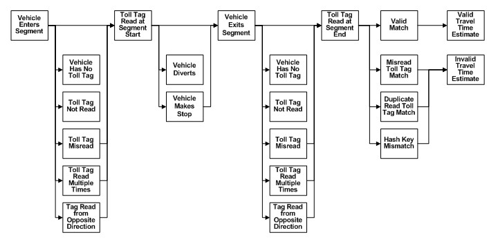
Figure 26. The Process for Estimating Travel Times from Toll Tag Readings

Each of these factors is described in the list below.

The effectiveness of a toll tag travel time system may be limited by a number of factors, including the fraction of vehicles equipped with toll tags, the effectiveness of the toll tag readers, duplicate reads, vehicle diversions and stops, and mis-matched tag reads.

• Vehicle Has No Toll Tag. The fraction of vehicles with toll tags was a critical factor in whether toll tag readers were an efficient approach for estimating travel times. Field tests conducted by FDOT prior to deciding to use toll tag readers for travel time estimation indicated that about 20 percent of vehicles in the Orlando area, which has a large number of toll roads, were equipped with toll tags. The proportion of vehicles with toll tags was lower in other parts of the state with fewer toll roads. The primary effect of this factor would be to reduce the number of tag reads that were available for making travel time estimates. An approach for mitigating against negative impacts would be to only use toll tag travel time systems in areas where the toll tag market penetration was high.
• Toll Tag Not Read. When optimally positioned, as at a toll booth, toll tag readers reliably read most tags. On Orlando arterials, the toll tag readers were placed roadside rather than directly overhead. This placed the readers further from the vehicles, reducing the efficiency with which they capture tag information. The readers were also aimed at a single lane of traffic and would read tags most effectively from that lane. Toll tags on vehicles in adjacent lanes would be read less efficiently. If a reader was not aimed correctly (e.g., was aimed between lanes, was aimed so that obstructions existed between the antenna and the vehicles), its read efficiency was lessened.
• Toll Tag Misread. It would be possible for a toll tag reader to misread a tag. Because of the error detection and correction capabilities built into toll tag readers, this type of error would be rare and should have little impact on toll tag travel time systems.
• Toll Tag Read Multiple Times. Most toll tag readers were designed for toll booth operations, where the sensors can be placed to detect toll tags in a limited area while a vehicle passess underneath the sensor. When deployed on iFlorida arterials, the readers were placed further from the vehicles and had a broader detection footprint. This increased the chance that a toll tag would be read more than once while passing through the detection zone. This effect was exacerbated if vehicles stopped in the detection zone - say, because a preceding vehicle was making a turn. Because of this possibility, a toll tag travel time system should include steps to identify and discard duplicate reads. For the iFlorida tag readers, duplicate reads accounted for between 5 and 10 percent of reads at most readers.
• Tag Read from Opposite Direction. Because iFlorida roadside toll tag detectors were angled across the lanes of traffic, it was possible that toll tags from some vehicles traveling in lanes for the opposite direction of travel were detected. In general, such detections should have little effect on toll tag travel times since there would not be a matching toll tag read upstream. If a vehicle turned around after being falsely detected, it could result in a travel time estimate that included the time spent turning around. One could mitigate against tag reads from the opposite direction of travel by comparing reads from detectors for each direction of travel and filtering out those that matched. FDOT relied on methods for excluding outliers for removing travel times computed from such reads.
• Vehicle Diverts. A vehicle that entered a travel time segment might fail to exit the segment because it diverted onto another route. On limited access highways, diversion opportunities would be limited. On arterials, there would be many opportunities to turn off of the travel time segment. The effect of vehicle diversions would be to reduce the fraction of vehicles entering a travel time segment that generated a travel time measurement by exiting the segment at its endpoint. One could reduce the opportunity for diversions to occur by using shorter travel time segments. With the iFlorida deployment, the effect of vehicle diversions was indicated by the fact that, with long travel time segments, few of the vehicles that entered a segment later exited that segment.
• Vehicle Makes Stop. A vehicle that entered a travel time segment might exit the segment, but do so after making an intermediate stop or a side-trip. As with vehicle diversions, this would be much more likely to occur on arterials than on limited access highways. The effect of a vehicle making a stop would be to produce a travel time measurement that was too long because it included the time the vehicle spent stopped. A sign of this in the iFlorida data was that the mean of all travel time measurements was typically much higher than the median. FDOT used algorithms to identify and remove outliers from the measured travel times.
• Duplicate Read Toll Tag Match. If duplicate tag reads were not filtered out when read, then the duplicates could result in associating multiple travel time measurements with the same trip - N duplicate reads at the starting point and M duplicate reads at the ending point could make a single trip appear as N times M travel time measurements. One potential effect if this occurred would be to bias the travel time estimates - slow moving vehicles would be more likely to generate multiple reads of longer travel times. One mitigation strategy would be to remove the duplicates before they enter the travel time calculation process.
• Hash Key Mismatch. In order to protect the privacy of the toll tag owners and the security of the toll tag IDs, the iFlorida AVI readers did not transmit the toll tag ID directly to FDOT. Instead, the reader produces a hash key that is related to the toll tag ID. Because the same hash key could be generated from two different toll tag IDs, it is possible that the hash key value of a vehicle entering a travel time segment could match the hash key value of a different vehicle exiting the segment. In the iFlorida deployment, the hash key values are six digit numbers, so that the frequency of hash key mismatches should be very low. If a mismatch did occur, the outlier removal process should prevent them from impacting the travel time estimates.

Other potential failure modes were associated with the specific process used in the iFlorida deployment to estimate and make use of travel times from toll tag readings (see Figure 27).

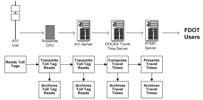
Figure 27. The iFlorida Toll Tag Travel Time Process

A toll tag travel time system should accommodate many different types of failures that might occur, including reader failures, clock mis-synchronization, incorrect reader location assignments, and network failures.

This process worked as follows. A toll tag was read from a vehicle passing one of the iFlorida toll tag readers and the data from that read was transmitted to a roadside central processing unit (CPU). This CPU accumulated readings from all readers deployed at a single site, archived those reads onto a local hard disk, and transmited each read to a central server. The roadside CPU also tracked transmissions that failed to reach the central server so that it ccould retransmit them at a future time. The central server batched all of the reads received during each one-minute interval, archived these one-minute batches, and transmited them to the travel time server. The travel time server combined each batch of data with other data previously received, matched toll tag reads across links to produce travel time measurements, excluded outliers from these measurements, and calculated the average travel time from the remaining measurements. The resulting travel time measurements were transmitted to the RTMC software, which used the travel times to support traffic management activities (e.g., produce automated 511 travel time messages) and archived the travel times in a data warehouse. The following list summarizes some failures that occurred as part of this specific toll tag travel time process.

• AVI Unit Failure. When the AVI unit failed, it produced fewer toll tag reads than expected, resulting in fewer travel time measurements. Early in the deployment, FDOT experienced significant problems with AVI unit failures (see section 3). Later, FDOT adopted an active monitoring program that included periodic comparison of the number of reads produced by each AVI unit with the expected number of reads to more quickly identify failed units. The presence of network addressable system diagnostics on the roadside CPU helped FDOT remotely check on the AVI status.
• Roadside CPU Failure. When the roadside CPU failed, then toll tag reads were not transmitted upstream in the travel time process and, depending on the type of failure, were not archived. In most cases, a CPU failure would prevent the roadside unit from operating. During iFlorida operations, two other types of failures occurred that made it appear that the roadside unit was operating, though the tag reads from the unit were not useful for generating travel time estimates.
  • One type of roadside CPU failure that occurred in the iFlorida system was that the clocks in the roadside CPUs did not remain synchronized. Since travel times were computed by comparing the timestamps between toll tag reads made by different readers, any discrepancy between the clocks on different roadside readers directly impacted the estimated travel times. One symptom of this type of failure was a discrepancy between the time stamps when a toll tag was read and when it was logged at the AVI server.
  • Another type of roadside CPU failure that occurred in the iFlorida system was the incorrect assignment of AVI units to device IDs when connecting AVI units to the roadside CPU. In the iFlorida system, the device ID was assigned by the roadside CPU according to the physical connection to which the AVI unit was connected. With up to four AVI units connecting to a roadside CPU, it sometimes happened that an AVI unit would be connected to the wrong physical connection on the CPU. This might mean that data for vehicles traveling northbound would be processed by the travel time server as if they were southbound vehicles, resulting in very low toll tag match rates and unusual travel times.
• Network Failure Between the Roadside CPU and the AVI Server. If the network failed between the roadside CPU and the AVI server, then the roadside CPU would continue to archive the toll tag reads, but the data would not be available to produce travel times. FDOT sometimes used the Ping command to determine they had network connectivity to field devices.
  • A secondary failure sometimes occurred in the iFlorida system when a roadside CPU was reconnected to the network after an outage. During the outage period, the roadside CPU would continue to archive toll tag reads. When reconnected to the AVI server, the roadside CPU would attempt to transmit the archived toll tag reads to the server, creating high demands on the server that would sometimes interrupt real-time data from other roadside CPUs. While this characteristic was key to supporting a toll system - lost toll tag information would mean lost revenue - it was a detriment in a real-time travel time system. When designing a toll tag travel time system, one should weigh the advantages of obtaining a more complete archive of toll tag reads (e.g., for back-computing travel times from archived data to fill in travel time information in the data warehouse when real-time travel time calculations were interrupted) with the disadvantages of potentially disrupting real-time travel time calculations.
  • Another related problem occurred during iFlorida operations, when some roadside CPUs re-transmitted toll tag reads to the AVI server several days after the initial transmission. This affected overall system performance by using up system resources transmitting redundant data, and also tainted the archives with the redundant data.
• AVI Server Failure. If the AVI server failed, then toll tag data was not transmitted to the travel time server and no real-time travel times were produced. Also, the toll tag data was not archived, though the data was often archived later when the AVI server became available and the roadside CPU's began transmitting their local archives of the toll tag data. With the iFlorida design, an AVI server failure would result in the loss of toll tag travel time estimates. FDOT considered installing a hot-swappable backup server available in case the AVI server failed. An alternate approach would be to include in the design of the RTMC server alternate approaches for entering travel time data for failed services. For example, the RMTC server could default to historical averages if the AVI server failed and allow RTMC operators to adjust these values manually (or disable them) if current conditions were significantly different from historical averages (e.g., when an incident occurs). This approach would serve as mitigation for any failure that might occur in the AVI travel time system.
• Network Failure Between the AVI Server and the Travel Time Server. The symptoms of this failure would be toll tag readings archived at the AVI server, but the lack of toll tag readings at the travel time server. If this occurred, no real-time travel time estimates would be generated. Possible mitigation strategies would be those typically used to improve network reliability, such as loops that provide redundant network paths between equipment. In the case of the iFlorida system, this network connection was made more complicated by the fact that the AVI server was part of the FDOT ITS network and the travel time server was on the OOCEA network.
• Travel Time Server Failure. A failure in the travel time server would prevent the generation of real-time travel time estimates. The possible mitigation strategies would be similar to those of the AVI server - a backup server and/or an alternate means of providing travel time data to the RTMC server.
• Network Failure Between the AVI Server and the Travel Time Server. A failure of this network connection would prevent the receipt by the RTMC server of the real-time travel time estimates produced by the travel time server.
• RTMC Server Failure. Because the RTMC server is the main software used to support RTMC activities, it was a critical system and included strongly protected against failure with power backup and a redundant, hot-swappable server. Failure of the RTMC server is outside the scope of a discussion of the toll tag travel time system.
  • The original iFlorida RTMC software, the Condition Reporting System, did exhibit one failure mode that directly related to the toll tag travel time system. In some cases, travel times produced by the toll tag travel time system would be combined for presentation as traveler information. For example, travel time estimates for all of the segments on SR 417 were summed to provide travel time comparisons for driving through Orlando on the two alternate routes available, I-4 and SR 417. When the CRS contractor originally configured the system, they created the wrong relationship between the travel time segments and the traveler information - travel times on SR 417 were being computed by summing travel times on the wrong segments. A number of factors helped lead to this failure, including a complex configuration process that made introduction of errors more likely and inadequate testing of the configuration data before it was put into use.

4.2. The iFlorida Toll Tag Travel Time Network

The development of the iFlorida toll tag travel time network began with studies to test the feasibility of using toll tag reads to measure travel times on Florida roads. One study¹ reported on field tests conducted on Florida Interstate highways. Field tests were conducted on urban portions of I-4 and I-95 and on rural portions of I-10, I-75, and I-95. These tests indicated that toll tag penetration was high in urban areas with toll roads, but was much lower in other areas:

Field studies can help determine if toll tag market penetration is sufficient to support the use of a toll tag travel time system.

• In Orlando, with five major toll roads (SR 408, SR 417, SR 429, SR 528, and the Florida Turnpike), almost 20 percent of vehicle on I-4 had toll tags.
• In Fort Lauderdale, with two major toll roads (the Florida Turnpike and the Sawgrass Expressway), about 10 percent of vehicles on I-95 had toll tags.
• In Tampa, with two toll roads (Lee Roy Selmon Expressway and Veterans Expressway), about 10 percent of vehicles on I-75 has toll tags.
• In St. Lucie County, with one major toll road (the Florida Turnpike), about 8 percent of vehicles on I-95 had toll tags.
• Brevard County has no toll roads, but is connected to Orlando by SR 528, which is tolled in Orange County. More than 6 percent of vehicles on I-95 in Brevard County had toll tags.
• In Jacksonville and Tallahassee, which have no nearby toll roads, about 1 percent of vehicles had toll tags.

Additional tests were conducted on Orlando arterials.² These tests showed a similar level of toll tag penetration in vehicles on Orlando arterials as observed on I-4 - toll tag reads were made for 15 to 20 percent of vehicles at the eight observation sites considered in the study. This report also identified the following information about the percent of reads at a station for which a matching read was identified at a second station, so that a travel time estimate could be made.³

• For SR 50 from Clarke Road to Good Homes Road (0.95 miles), about 53 percent of toll tag reads resulted in a travel time estimate.
• SR 50 from Goldenrod Road to Old Cheney Highway (1.2 miles), about 54 percent of toll tag reads resulted in a travel time estimate.
• SR 436 from US 17/92 to Maitland Avenue (1.5 miles), about 48 percent of toll tag reads resulted in a travel time estimate.
• SR 436 from Curry Ford Road to Lee Vista Blvd (3.6 miles), about 30 percent of toll tag reads resulted in a travel time estimate.

For the segments considered in this study, the toll tag readers generated between 10 and 20 travel time estimates per hour. Based on this information about the feasibility of using toll tag readers to estimate travel times on Orlando arterials and limited access roads, FDOT developed a plan for doing so. The locations of the toll tag readers is depicted in Figure 3 on page 5, with the resulting travel time segments listed in Table 2.

Table 2. iFlorida Arterial Travel Time Segments

Road	Segment	Length (miles)	Lanes	Major Intersections	Volume
SR 50 (Colonial Dr)	SR 91 to SR 429	4.9	2	7	28,500 to 50,000
SR 50 (Colonial Dr)	SR 429 to SR 408	2.4	2	4	56,000 to 44,500
SR 50 (Colonial Dr)	SR 408 to SR 423	6.5	3	17	33,500 to 47,500
SR 50 (Colonial Dr)	SR 423 to SR 441	1.1	3	3	47,500 to 36,500
SR 50 (Colonial Dr)	SR 441 to I-4	0.8	2	3	41,500 to 44,500
SR 50 (Colonial Dr)	I-4 to US 17/92	1	2	4	44,500 to 43,000
SR 50 (Colonial Dr)	US 17/92 to SR 436	3.4	3	12	48,000 to 65,000
SR 50 (Colonial Dr)	SR 436 to SR 417	3	3	4	45,500 to 44,500
SR 50 (Colonial Dr)	SR 417 to SR 408	4.5	3	8	53,500 to 45,500
SR 414 (Maitland Blvd)	SR 441 to I-4	4.3	3	2	31,000 to 66,500
SR 414 (Maitland Blvd)	I-4 to US 17/92	2	2	7	56,000 to 31,500
SR 423 (John Young Parkway) (Lee Rd)	SR 417 to SR 528	2.8	3	3	(no data)
SR 423 (John Young Parkway) (Lee Rd)	SR 528 to I-4	6.1	3	3	(no data)
SR 423 (John Young Parkway) (Lee Rd)	I-4 to SR 408	3	3	3	(no data)
SR 423 (John Young Parkway) (Lee Rd)	SR 408 to SR 50	0.7	3	3	48,000 to 49,000
SR 423 (John Young Parkway) (Lee Rd)	SR 50 to SR 441	3.2	2	2	46,500 to 40,500
SR 423 (John Young Parkway) (Lee Rd)	SR 441 to I-4	2.1	3	3	38,500 to 44,500
SR 423 (John Young Parkway) (Lee Rd)	I-4 to US 17/92	1.3	2	2	40,500
SR 436 (Semoran Blvd)	SR 441 to SR 434	5.4	4	12	23,000 to 48,500
SR 436 (Semoran Blvd)	SR 434 to I-4	1.8	4	7	48,500
SR 436 (Semoran Blvd)	I-4 to US 17/92	3.1	4	12	63,000 to 62,000
SR 436 (Semoran Blvd)	US 17/92 to SR 50	7.9	3	19	70,500 to 52,000
SR 436 (Semoran Blvd)	SR 50 to SR 408	1.2	3	3	55,000 to 52,500
SR 436 (Semoran Blvd)	SR 408 to SR 528	5.4	3	13	57,000 to 42,000
SR 441 (Orange Blossom Trail)	US 192 to SR 417	4.7	3	7	30,500 to 34,500
SR 441 (Orange Blossom Trail)	SR 417 to SR 528	4.4	3	8	50,500 to 42,000
SR 441 (Orange Blossom Trail)	SR 528 to I-4	4.7	3	13	61,500 to 66,500
SR 441 (Orange Blossom Trail)	I-4 to SR 408	2.2	2	5	36,500
SR 441 (Orange Blossom Trail)	SR 408 to SR 50	1.2	2	7	36,500 to 28,500
SR 441 (Orange Blossom Trail)	SR 50 to SR 423	3.4	2	4	32,500 to 31,000
SR 441 (Orange Blossom Trail)	SR 423 to SR 414	3.4	2	4	35,000 to 33,000
SR 441 (Orange Blossom Trail)	SR 414 to SR 436	3.5	2	5	33,000 to 27,000
SR 441 (Orange Blossom Trail)	SR 436 to SR 429	2.2	2	4	41,500 to 38,000
US 192 (West Coast Parkway)	I-4 to SR 441	9.8	3	18	54,000 to 37,000
US 192 (West Coast Parkway)	SR 441 to SR 91	3.6	3	9	35,500 to 36,000
US 17/92 (Orlando Ave)	SR 50 to SR 423	2.7	2	9	28,000 to 37,500
US 17/92 (Orlando Ave)	SR 423 to SR 414	2.3	3	4	45,500 to 33,500
US 17/92 (Orlando Ave)	SR 414 to SR 436	1.9	3	2	61,000 to 55,500
US 17/92 (Orlando Ave)	SR 436 to SR 417	8.8	3	15	60,500 to 43,500

In this table, the Road column identifies the road on which each travel time segment lies with the segments, running either from East to West or from South to North, identified by the cross-streets bounding each segment. The length of the segment and the number of lanes was provided by FDOT. The number of intersections column lists the number of major intersections within each segment (i.e., excluding the intersections at the start and end of each segment), where each interchange and each intersection with a stop bar was identified as a major intersection. The volume information was obtained from FDOT statewide traffic count.⁴

Table 3 lists similar information for the FDOT toll tag travel time segments on limited access highways and on evacuation routes where travel time were monitored by either toll tag or license plate readers.

Table 3. iFlorida Limited Access and Evacuation Travel Time Segments

Road	Segment	Length (miles)	Lanes	Major Intersections	Volume
SR 91 (The Florida Turnpike)	US 192 to SR 522	4.2	2	0	32,800
SR 91 (The Florida Turnpike)	SR 522 to SR 528	6.9	2	0	32,800 to 41,700
SR 91 (The Florida Turnpike)	SR 528 to I-4	4.1	2	0	41,700 to 44,700
SR 91 (The Florida Turnpike)	I-4 to SR 408	6.1	2	0	44,700
SR 91 (The Florida Turnpike)	SR 408 to SR 50	7	2	1	44,700 to 48,100
SR 417	I-4 to Boundary	5.1	2	2	10,200 to 16,300
SR 417	Boundary to SR 434	6.1	2	2	45,000 to 28,800
SR 417	SR 434 to US 17/92	6.6	2	1	24,100 to 14,500
SR 417	US 17/92 to I-4	4.8	2	2	(no data)
SR 520	SR 528 to I-95	13.9	1	2	(no data)
SR 528	I-4 to SR 91	4.3	2	3	60,600 to 54,400
SR 528	SR 91 to Boundary	4.6	2	0	54,400 to 49,800

4.3. The iFlorida Toll Tag Travel Time Estimation Process

As each toll tag reader observed toll tag IDs on passing vehicles, it transmited an encrypted hash key representing that ID along with the time it was observed to a Travel Time Server. This server matched toll tag observations made at readers at the start and end of each travel time segment to generate travel time measurements. Anomalous measurements were discarded, and the remaining measurements were used to estimate the average travel time, using one of two possible approaches. In the first approach, a rolling average of recent observations over a fixed period of time was used. This approach was used when travel time observations were plentiful. In the second approach, a rolling average of the most recent fixed number of observations was used. This approach was used when fewer observations were available. Within this general framework, a number of configurable parameters were used to control the specific operations of the process.

• The Tag-Discard-Horizon parameter controled the time an unmatched tag read was kept "in the system" before discarding it. This parameter set a de facto upper bound on the maximum travel time that could be observed by the system.
• The Maximum-Speed-Threshold was used to prevent reporting of travel times indicating that current travel speeds were higher than the speed limit. If the travel speed associated with a travel time observation was greater than this amount, the travel time was adjusted upward so as to result in a travel speed equal to this parameter.
• The Speed-Threshold parameter was used to remove anomalous travel time observations. If the travel speed associated with a travel time observation differed from the last estimated average travel time by this amount or more, it was discarded.
• The Link-Threshold parameter was used to remove anomalous travel time observations. If the percentage change in either the travel time observation or the associated travel speed relative to the last estimated average travel time / travel speed was greater than this amount, it was discarded.
• The Anomaly-Threshold parameter was used to remove anomalous travel time observations. If the travel speed associated with a travel time observation was greater than this amount, it was discarded. This parameter set a minimum for travel time observations.
• The Time-Window parameter specified the time interval over which travel times were averaged when the first averaging approach was used.
• The Sample-Size parameter specified the number of observations that were averaged when using the second averaging approach.
• The FM2-Timeout parameter specified the maximum time over which travel times were averaged when using the second averaging approach.
• The Time-Slice parameter specified the frequency with which the travel time calculations were performed.

This travel time process was originally designed for computing travel times for OOCEA on limited access toll highways, and the configuration parameters were set to the default values used on those highways. A number of adjustments were made to try to optimize the parameters for use on Orlando arterials.

4.4. An Example – Toll Tag Travel Time Estimates on Colonial Drive

This section exemplifies the performance of the toll tag travel time system by examining its performance on the eastbound section of Colonial Drive between US 17/92 (Mills Avenue) and SR 436 (Semoran Boulevard). This helps lay the groundwork for a more general analysis of the entire network by identifying performance characteristics that should be considered in the more general analysis.

Table 2 indicates that this section of road is 3.4 miles long, has 3 lanes in each direction of travel, includes 12 major intersections, and has a traffic volume ranging from 48,000 vehicles per day at the western portion of the section to 65,000 vehicles per day at the eastern portion of the section. The configuration of the intersection at the start of this travel time link is depicted in Figure 28.

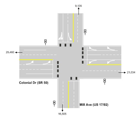
Figure 28. The Intersection of SR 50 and US 17/92

In this figure, the numbers are intersection traffic counts from City of Orlando traffic count program and the icons beside the roads represent the approximate location of the toll tag readers. Figure 29 depicts the configuration of the intersection at the end of this travel time link.

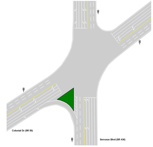
Figure 29. The Intersection of SR 50 and SR 436

Not shown in this figure is a road leading from SR 50 west of SR 436 to SR 436 southbound, which serves as a de facto turn lane for eastbound traffic on SR 50 wishing to turn right onto SR 436.

The iFlorida travel time process for this travel time segment matched reads from the toll tag reader monitoring eastbound traffic on SR 50 east of the US 17/92 intersection with those from the reader monitoring eastbound traffic on SR 50 east of SR 436. (An alternate approach would be to include reads from the three readers at the SR 50 / SR 436 intersection monitoring eastbound traffic on SR 50 and north- and south-bound traffic on SR 436, though this approach would mix travel times that did and did not include the additional delay associated with making a left turn from SR 50 onto SR 436.) The number of tag reads at the SR 50 Eastbound, East of US 17/92 reader are depicted in Figure 30 (for weekdays) and Figure 31 (for weekends).

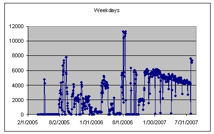
Figure 30. Weekday Tag Reads at the SR 50 Eastbound, East of US 17/92 Reader

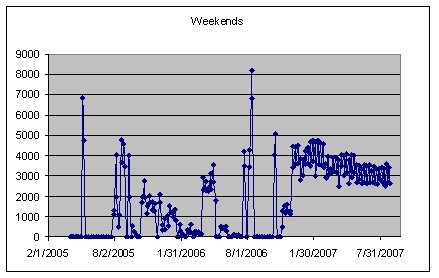
Figure 31. Weekend Tag Reads at the SR 50 Eastbound, East of US 17/92 Reader

Note that this reader first began operating stably in December 2006. Prior to that time, the reader often had no tag reads or fewer reads than should have been expected. Once it began operating stably, the number of reads per day remained between 4,000 and 6,300 on most weekdays and between 2,500 and 5,000 on most weekend days. The period in early August 2006 when more reads than usual were observed occurred when the reader re-transmitted the toll tag reads that occurred on August 1 and 2, 2006. After December 2006, the reader operated with only four days of very few reads and nine days with fewer reads than expected, but still sufficiently many to support travel time calculations.

Figure 32 is a frequency chart listing the number of days the reader at SR 50 Eastbound East of US 17/92 had a number of reads within a series of ranges for the period from 1/1/2007 through 8/26/2007. The lowest range category was 0 to 2,000 reads and the highest range category was more than 6,500 reads, with the size of each category in between being 250 reads.

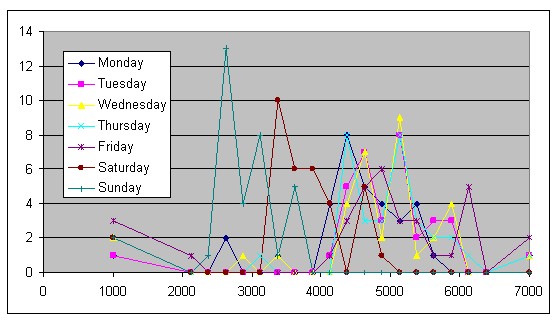
Figure 32. Toll Tag Reads at SR 50 Eastbound, East of US 17/92, by Day of Week

This indicates that the range for the number of reads per day was similar across weekdays, but different for Saturday and Sunday. Note that the average number of reads per day was about 4,500. Of these, about 500 reads per day were duplicate reads - multiple reads of the same tag at the same location within a five minute period - leaving about 4,000 vehicles read per day. Figure 28 indicates that the eastbound volume at the reader location was about 21,000 vehicles per day, indicating that the reader was identifying about 19 percent of the passing vehicles. This was consistent with the observations made by FDOT prior to the iFlorida deployment.

Another measure of the operational status of a reader for supporting travel time calculations was the lag time between when a toll tag read was made and when it reached the toll tag server. Figure 33 depicts the measured lag time for the SR 50 Eastbound, East of US 17/92 reader.

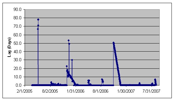
Figure 33. Lag Time for the SR 50 Eastbound, East of US 17/92 Reader

Because the lag time was measured as the difference between when a reading was timestamped by a roadside CPU and when it was logged at the AVI server, there were several possible causes for a lag:

• The clocks on the roadside CPU and the AVI server were different. In this case, the apparent lag should be relatively constant over time until the clocks were reset.
• The roadside CPU lost network connectivity to the AVI server for a time and, when connectivity was restored, uploaded the archived data that could not be sent to the server while connectivity was unavailable. In this case, the apparent lag should decrease over time at a rate of a bit less then one day of lag per day. The period in the above figure from October 31, 2006 through December 31, 2006 is an example.
• The roadside CPU could have re-transmitted data at a later date, duplicating data that had already been transmitted. In this case, the apparent lag should decrease over time at a rate of roughly half day of lag per day and the number of reads (see Figure 30) should be significantly higher than usual. The period in the above figure from August 1, 2006 through August 15, 2006 is an example.

Based on the number of reads and the lag time, a value representing the operational status of the reader was assigned to the reader for each day. The following codes were used:

• A value of "6" was used if a toll tag reader generated no reads. This probably indicates that the toll tag reading hardware was not operating correctly.
• A value of "5" was used if a toll tag reader generated data, but the lag time was high and decreasing at a rate of about one day of lag per day. This probably indicates that the reader had lost network connectivity to the AVI Server.
• A value of "4" was used if a toll tag reader generated data and the lag time was high, but did not following the pattern of decreasing one day of lag per day. This could indicate that the clocks on the roadside CPU and the AVI Server were not synchronized or that data was being re-transmitted.
• A value of "3" was used if a toll tag reader was generating fewer than 500 reads per day. This could indicate a problem with the toll tag reader, and meant that the reader was generating too few reads to be useful for supporting travel time calculations.
• A value of "2" was used if the reader was generating significantly fewer reads than usual, but still more than 500 reads per day. This could indicate a problem with the toll tag reader, or could just be a side effect of unusual traffic conditions for that day.
• A value of "1" was used if the reader generated significantly more reads then expected. This could be caused by a reader re-transmitting toll tag data, or by unusual traffic conditions.
• A value of "0" was used if none of the above deficiencies were noted.

The following four figures depict the operational status of each toll tag reader associated with the travel time segment on SR 50 from US 17/92 to SR 436. Note that a maximum value of 0 or 1 indicates that the reader was 100 percent operational from the standpoint of computing travel times, a value of 2 indicates that the reader was operating at lower effectiveness, and that higher values indicate that the reader could not be used to provide real-time travel times.

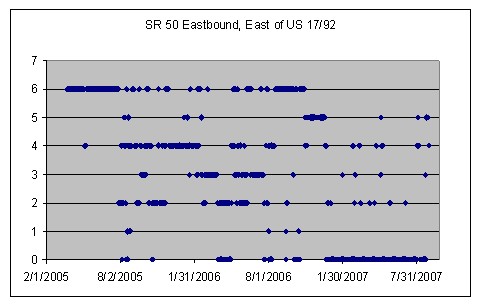
Figure 34. Errors at the SR 50 Eastbound, East of US 17/92 AVI Reader

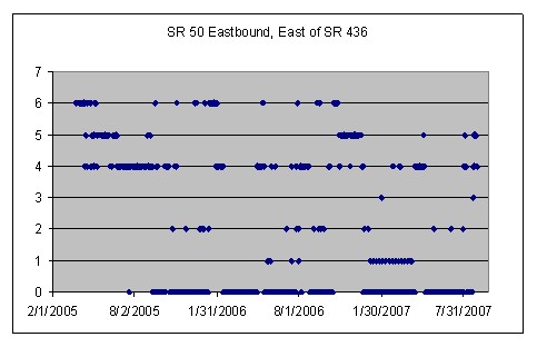
Figure 35. Errors at the SR 50 Eastbound, East of SR 436 AVI Reader

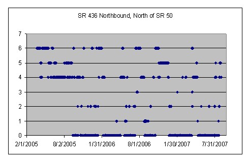
Figure 36. Errors at the SR 436 Northbound, North of SR 50 AVI Reader

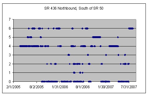
Figure 37. Errors at the SR 436 Southbound, South of SR 50 AVI Reader

Figure 38 combines the error information for the above four readers to identify the operational status of the travel time system for the travel time segment, with a value of 100 percent being used if the three readers used for the travel time calculation were all fully operational and lower percentages being used to represent degraded performance if one or more of the readers was exhibiting one or more deficiencies.

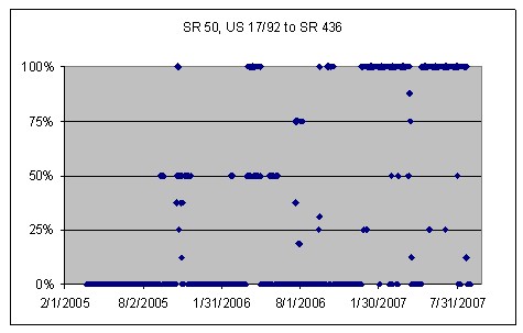
Figure 38. Status of the Travel Time System for SR 50 from US 17/92 to SR 436

Figure 39 summarizes this data by computing the average percent operational for each month.

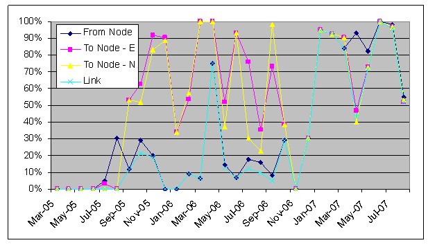
Figure 39. Monthly Status of the Travel Time System for SR 50 from US 17/92 to SR 436

Together, the above charts and figures provide measures for assessing the operational status of the portion of the toll tag reader network needed to support travel time estimates for the travel time segment on SR 50 from US 17/92 to SR 436. They indicate that, prior to 2007, the network was unreliable. Over the first eight months of 2007, the system was above 90 percent operational in four months, with lower levels of reliability in the other months.

But, the operational status of the toll tag reader only tells part of the story of a toll tag travel time network. Because the iFlorida arterial travel time segments were long with many opportunities for travelers to divert, it was possible that many travelers entering the segment did not exit it at its endpoint. The percentage of (non-duplicated) toll tag reads for vehicles entering the travel time segment during the period from August 13, 2007 to August 19, 2007 are listed in Table 4. (That time period was chosen because the readers for this travel time segment did not exhibit any deficiencies on those days.)

Table 4. Matching Effectiveness for the SR 50 from US 17/92 to SR 436 Segment

Date	Duplicate Reads	Non-Matching Reads	Matching Reads	Matching Percent
8/13/2007	345	3,165	612	16.20%
8/14/2007	319	3,262	610	15.80%
8/15/2007	421	3,265	692	17.50%
8/16/2007	373	3,350	690	17.10%
8/17/2007	423	3,350	598	15.10%
8/18/2007	286	2,787	496	15.10%
8/19/2007	149	2,321	440	15.90%

This table indicates that, for this travel time segment, about 16 percent of the toll tag reads made at the start of the segment would result in travel time measurements. However, some of these measurements may be invalid. For example, if a traveler makes a stop mid-segment, then later completes the segment, the result would be a travel time measurement that included the time the traveler spent stopped. This was more problematic for arterials than limited access highways because stops were more likely to occur and, if a stop occurred, it was more difficult to differentiate between a stop-induced delay and a delay induced by traffic signals encountered while traveling the segment. Figure 40 depicts the distribution for the travel times observed during the period from Monday August 13, 2007 through Friday August 17, 2007.

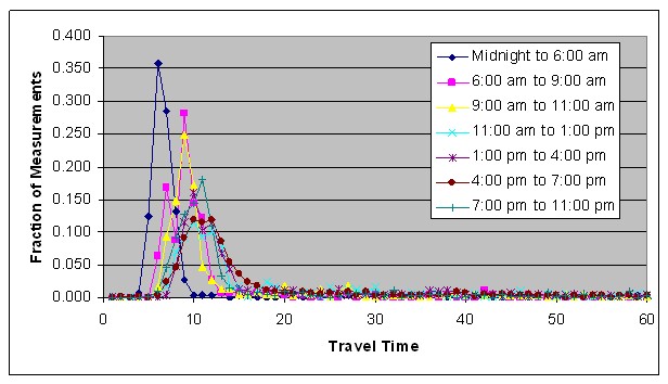
Figure 40. Travel Time Distribution for the SR 50 from US 17/92 to SR 436 Segment

The important thing to note about these distributions is the long tail of high travel times, indicative of travel times that include time spent stopped or diverting. The effect of these outliers on the mean travel time is shown in Table 5.

The effect of diverting traffic on arterials can introduce a high bias into the observed average travel time.

Table 5. Travel Time Statistics for the SR 50 from US 17/92 to SR 436 Segment

Time Period	Count	Median	Mean	Percent Outlier
Midnight to 6:00 am	257	6.1	7.4	5%
6:00 am to 9:00 am	263	8.8	10.3	5%
9:00 am to 11:00 am	319	9	14	18%
11:00 am to 1:00 pm	375	12.2	22.5	25%
1:00 pm to 4:00 pm	665	11.5	20.9	23%
4:00 pm to 7:00 pm	700	11.8	19.4	19%
7:00 pm to 11:00 pm	533	10.4	17.6	17%

In this table, the Percent Outlier column indicates the percentage of high travel time measurements that should be discarded as outliers in order for the corrected mean (i.e., mean for measurements after outliers are removed) to equal the median. Note that, without correcting for the outliers, the mean is a poor estimator of the travel time experienced by most travelers. Based on this example, it appears that the median may be a better choice for estimating the segment travel time based on arterial probe measurements than the mean. If the mean is used, a method for removing high travel time outliers resulting from intermediate stops and diversions must be used.

For limited access highways, diverting traffic is less likely to introduce a high bias into the observed average travel time.

For comparison, Figure 41 and Table 6 show corresponding travel times for a limited access section of highway, SR 417 from I-4 north of Orlando to US 17/92.

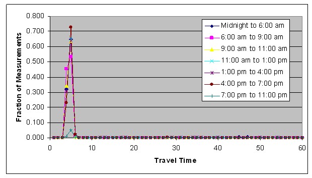
Figure 41. Travel Time Distribution for the SR 417 from I-4 to US 17/92 Segment

Table 6. Travel Time Statistics for the SR 417 from I-4 to US 17/92 Segment

Time Period	Count	Median	Mean
Midnight to 6:00 am	153	4.1	4.7
6:00 am to 9:00 am	869	4	4.3
9:00 am to 11:00 am	307	4.1	4.7
11:00 am to 1:00 pm	218	4.1	5.2
1:00 pm to 4:00 pm	441	4.1	5.3
4:00 pm to 7:00 pm	751	4.2	4.8
7:00 pm to 11:00 pm	298	4.1	4.7

Note that, for the limited access highway, outliers with travel time significantly above the median value were much less common and the mean and median were relatively close to each other in value.

Another question related to the effectiveness of a toll tag travel time system was whether it will generate enough toll tag matches to produce reliable travel times. Figure 42 depicts the average number of travel time reads per hour for the SR 417 from I-4 to US 17/92 segment during the period from August 13, 2007 to August 17, 2007.

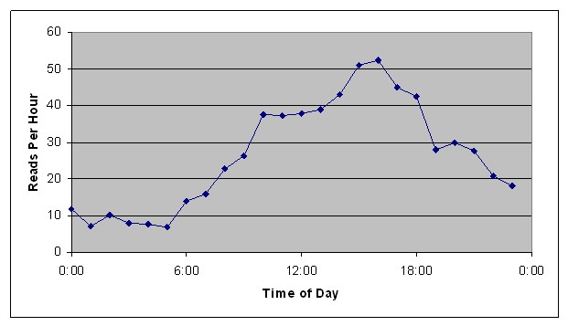
Figure 42. Travel Times Per Hour for the for the SR 417 from I-4 to US 17/92 Segment

The following approach can be used to generate a rough estimate of the number of travel time measurements needed to generate an accurate estimate for the average travel time. The curves in Figure 40 indicate that the width of the travel time distributions is roughly equal to the median, which is roughly equal to the mean after the top 25 percent of measurements are removed as outliers. Under these circumstances, a sample size of 25 (after removing outliers) would result in an estimate of the mean travel time that should be within 15 percent of the actual value about 90 percent of the time. A sample size of about 32 would provide enough measurements so that, after removing outliers, a sample size of 25 would remain. During peak hours, it required more than 30 minutes to accumulate 32 travel time measurements. During night time hours, it required about 3 hours to accumulate 32 travel time measurements. On weekends, when traffic volumes are lower, longer accumulation times would be needed.

These observations pointed to a tradeoff that must be considered when designing an arterial toll tag travel time system. If one assumes that the travel times do not change significantly over time, then averaging over a long time period will increase the number of observations over which the average is taken, which increases the statistical accuracy of the estimate for the mean travel time. If travel times do change over time, averaging over a long period of time would include in the average travel times that no longer represent current travel time conditions. This is exemplified in Figure 43, which depicts travel times on the SR 50 from US 17/92 to SR 436 travel time segment during the period from 6:00 pm to 7:00 pm on August 13, 2007, a time during which travel times were decreasing as rush hour ended. (Travel times greater than 20 minutes have been excluded from this chart.)

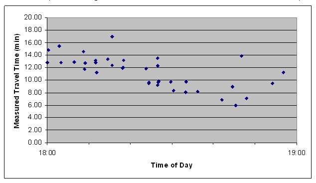
Figure 43. Travel Times for SR 50 from US 17/92 to SR 436 on 8/13/2007

Figure 44 shows the average travel times computed from the observed travel times on this day, using different values for the length of the interval (i.e., the lag time) over which the average was computed.

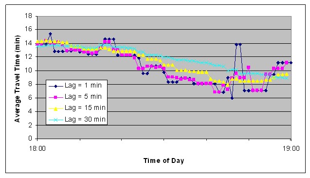
Figure 44. Average Travel Times for SR 50 from US 17/92 to SR 436 on 8/13/2007

Note that, as the lag time increased, the travel time curve was smoother, but the average travel time was larger than the recently observed travel times because the average included observed travel times from further in the past when congestion levels were higher. This is generally true. Averaging over short periods of time will result in highly variable estimates for the average travel time because the averages include few observations. The situation would be much worse if traffic conditions changed more abruptly, as might occur if a crash occurred on the travel time segment.

The main problem was that there are relatively few observations - averaging about one observation every two minutes for the period in question. Averaging over a short period of time, so that the estimated travel times responded quickly to changes in traffic conditions, meant that the estimated travel times were based on very few measurements and the variability in the estimated travel times was high. Averaging over a longer period of time to reduce this variability dampened the response to changes in traffic conditions.

One way to improve the performance of the travel time system would be to increase the number of observations by allowing multiple toll tag readers to supply measurements at the end point of a travel time segment. In the example at hand, all vehicles entering the segment pass by the toll tag reader on SR 50 eastbound, east of US 17/92. Vehicles that turn onto SR 436 at the end of the segment do not pass by the reader on SR 50 eastbound, east of SR 436 - left-turning vehicle pass by the reader on SR 436 northbound, north of SR 50 and most right-turning vehicles do not pass by a reader because the reader location is north of the entry point taken by most right-turning vehicles. The Travel Time Server used for iFlorida only allows use of a single reader for the endpoint of a travel time segment. A tool developed by the Evaluation Team allowed multiple readers to be used at both the start and end point of a travel time segment. Table 7 summarizes results travel time results for the section of SR 50 from US 17/92 to SR 436 using different numbers of readers for the end node.

Table 7. Travel Time Statistics for the SR 50 from US 17/92 to SR 436 with Different End Node Configurations

End Node	Time Period	Raw Data			Corrected Data
		Match Count	Match Percent	Mean TT (min)	Match Count	Match Percent	Mean
SR 50 Eastbound and SR 436 Northbound	Midnight to 6:00 am	385	34%	8.3	273	24%	6
SR 50 Eastbound and SR 436 Northbound	6:00 am to 9:00 am	394	19%	11.1	314	15%	8.4
SR 50 Eastbound and SR 436 Northbound	9:00 am to 11:00 am	394	17%	12.8	329	14%	9.4
SR 50 Eastbound and SR 436 Northbound	11:00 am to 1:00 pm	449	13%	16.9	345	10%	11.6
SR 50 Eastbound and SR 436 Northbound	1:00 pm to 4:00 pm	831	16%	19	659	13%	11.6
SR 50 Eastbound and SR 436 Northbound	4:00 pm to 7:00 pm	925	19%	17.1	763	16%	11.5
SR 50 Eastbound and SR 436 Northbound	7:00 pm to 11:00 pm	710	21%	16	574	17%	10.3
SR 50 Eastbound Only	Midnight to 6:00 am	265	24%	8.2	168	15%	5.8
SR 50 Eastbound Only	6:00 am to 9:00 am	267	13%	10.8	209	10%	8.5
SR 50 Eastbound Only	9:00 am to 11:00 am	284	12%	12.5	231	10%	9.2
SR 50 Eastbound Only	11:00 am to 1:00 pm	326	9%	17.1	249	7%	11.5
SR 50 Eastbound Only	1:00 pm to 4:00 pm	609	12%	18.2	481	10%	11.3
SR 50 Eastbound Only	4:00 pm to 7:00 pm	646	13%	16.8	522	11%	11.5
SR 50 Eastbound Only	7:00 pm to 11:00 pm	506	15%	16.1	398	12%	10.4
SR 436 Northbound Only	Midnight to 6:00 am	151	13%	9	80	7%	6.2
SR 436 Northbound Only	6:00 am to 9:00 am	144	7%	12.3	101	5%	8.5
SR 436 Northbound Only	9:00 am to 11:00 am	122	5%	14.4	90	4%	10
SR 436 Northbound Only	11:00 am to 1:00 pm	149	4%	17.9	106	3%	12.8
SR 436 Northbound Only	1:00 pm to 4:00 pm	268	5%	21.8	199	4%	12.6
SR 436 Northbound Only	4:00 pm to 7:00 pm	333	7%	18.5	260	5%	11.5
SR 436 Northbound Only	7:00 pm to 11:00 pm	251	7%	16.4	179	5%	10.7

In this table, the corrected data was generated by excluding from the mean those travel time values that were more than 0.5 standard deviations above the mean. Note that including the northbound vehicles on SR 436 in the travel time calculation increased the number of travel time matches by almost 50 percent. This increase in the sample size could result in more reliable travel time estimates or allow for a shorter averaging period with the same level of reliability.

It is interesting to note that the two travel time measurements, one for vehicles going straight through the SR 50 / SR 436 intersection and one for those turning left, provide a measure of the additional delay - about 36 seconds - for vehicles that turn left at that intersection relative to those that go straight.

In summary, the review of toll tag travel time operations for the SR 50 eastbound, from US 17/92 to SR 436, travel time segment identified the following observations regarding the use of toll tag readers for arterial travel times:

• The toll tag reader recorded toll tag readings from about 20 percent of the passing vehicles.
• Duplicate reads accounted for about 10 percent of the reads at each reader. The travel time system should include methods for excluding such duplicate reads.
• Maintaining toll tag readers was difficult. From May 2005 (when the reader deployment was complete) and December 2006, the readers on this segment were seldom operational. During the first eight months of 2007, the system was capable of producing travel times about 80 percent of the time.
• About 16 percent of the toll tag readings made at the start of the travel time segment matched with toll tags at the end of the travel time segment, resulting in a travel time measurement.
  • This percentage could be boosted to about 24 percent if the readers monitoring vehicles that turn at the end intersection are included in the travel time calculation.
  • About 25 percent of the travel time measurements were high travel time outliers, most likely associated with travelers who make a stop mid-trip or divert onto another route and just happen to drive by the end-point toll tag reader at a later time. These outliers must be excluded if the average observed travel time is to be a reliable estimator for the travel time experienced by most travelers on an arterial. The median observed travel time might be a more reliable estimator.
  • It did not appear that there were a significant number of low travel time outliers - the outliers are likely caused by stops and diversions, which always increase travel times. An asymmetric method focused on excluding long travel time outliers should be used.
• The system did not produce enough travel time matches to produce reliable travel time estimates without accumulating travel time observations over a relatively long period—about 30 minutes during peak hours and up to 3 hours after midnight.

In the following sections, these factors will be examined on a system-wide basis.

4.5. Toll Tag Reader Operations

This section reviews the operation of the toll tag reader system, with the primary objective being to assess the reliability of the iFlorida toll tag reader network. The following list describes the primary measures were used to assess the level of service provided by the iFlorida toll tag readers. (Appendix A describes these measures in more detail.)

• The Level of Service for Tag Reads (LOS_Reads) indicates whether a reader was producing fewer tag reads than expected, with 0 indicating it was producing few if any reads and 1 indicating it was producing at least as many as expected.
• The Level of Service for Latency (LOS_Latency) indicates if the read tags were correctly timestamped and reached the toll tag server in a timely manner. A value of 0 indicates that either the data did not reach the toll tag server quickly enough to be used for real-time travel time calculations or the timestamps were to inaccurate to be used for travel times.
• The Reader Level of Service (LOS_Reader), which is the product of LOS_Reads and LOS_Reads, indicates if the number of reads and latency are both within expected operational bounds.

These measures were assessed for each iFlorida toll tag reader. Figure 45 summarizes this level of service information by presenting the weekly average for the level of service summed across all the iFlorida toll tag readers. Table 19 in Appendix A provides a more detailed listing of these measures for the toll tag readers on SR 50.

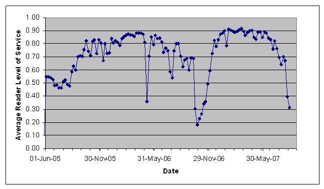
Figure 45. Weekly Average Level of Service for iFlorida Toll Tag Readers

Note that the deployment of the toll tag reader system was completed May 31, 2005, a time when the level of service was just above 50 percent. The main cause for the low level of service at this time was that the readers were actually deployed and tested from February through May 2005, but there was no regular monitoring of the status of the already tested equipment until August 2005. Many devices failed during this period. With so many devices failed, the maintenance contractor had neither the man-power nor the spare parts available to quickly make all the necessary repairs. The need for so many spare parts at the same time also overwhelmed the manufacturer, who was unable to promptly replace failed equipment.

It is important that a system to monitor and maintain field equipment be in place by the time any field equipment is deployed.

The challenge of maintaining the network was made more difficult because FDOT did not have access to a simple way to monitor the equipment. The contractor provided neither a tool nor instructions for monitoring the status of the toll tag readers. The CRS software, which displayed travel times produced by the readers, was having reliability problems of its own, preventing FDOT from using the lack of travel times in the CRS as an indicator of a failed toll tag reader. FDOT resorted to a manual process of reviewing the log files at the toll tag server to determine if a reader was producing toll tag reads and providing them to the server. This process, which initially required almost half a day to complete, is still in use today, though it has been refined and now only requires about one hour each day.⁵

By January 2005, FDOT had achieved a fairly high level of service for the readers. FDOT attributed the drop in the number of functioning readers that occurred at times during that year to failures due to lightening strikes, though network cuts also caused some failures. The high number of failures resulted in a long turn-around time in getting replacement parts, extending the downtime when a reader did fail. After noting the high number of lightening-induced failures, FDOT tested the use of power conditioners and new grounding methods to reduce these failures.

By January 2006, the level of service for the readers operated stably at about 90 percent for most of 2007 before the reliability dropped off again beginning in June 2007. When the warranty period for the readers ended in May 2007, FDOT did not receive adequate documentation or training on how to configure replacement parts. This delayed repairs, allowing failed units to accumulate while FDOT was conducting tests and developing repair procedures.

Reader failures will occur. The systems that rely on the readers must be designed to work around those failures.

Despite considerable effort and expense devoted to maintaining the toll tag reader network, the network averaged almost 10 percent failed readers when working well. At times, the failure rates were much higher. Because the CRS software did not include a graceful way of coping with missing travel time data resulting from these failures, such as filling in missing data with historical averages and alerting operators that historical averages were being used so that they can more closely monitor the affected segments, a failed reader usually resulted in missing travel information.

The reader level of service values provide an indication of how well each individual reader was operating. However, it requires reads fom two toll tag readers to generate a travel time estimate, so the level of service for a travel time segment should be a combination of the level of service values for the readers at the from and to nodes for that segment. The Segment Level of Service, LOS_Segmentprovides a measure of whether the travel time system is producing as many travel time estimates as usual. (This measure is defined in Appendix A.) Figure 46 depicts the level of service for the iFlorida toll tag travel time links.

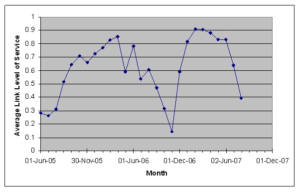
Figure 46. Monthly Average Level of Service for iFlorida Toll Tag Travel Time Links

Note that it closely follows the level of service chart for the toll tag readers, except that the level of service is generally lower. This is because the level of service for the travel time segment is lowered whenever the level of service of the readers at either node of the segment drops.

4.6. Toll Tag Matching Efficiency

Another factor that impacts the effectiveness of toll tag readers for estimating travel times is the efficiency of the toll tag matching - what fraction of tag reads at the entrance to a travel time segment result in a travel time estimate when the vehicle exits the segment. The following list describes the main factors that affect this efficiency.

• The number of entering vehicles exiting the segment before reaching the end. If an entering vehicle exits the segment before reaching the segment end, no travel time estimate will be produced. A number of variables could impact the number of vehicles that exit the segment before reaching the end.
  • The length of the segment. If a segment is longer, it will typically have more exit points along it and more vehicles will exit along it.
  • The number of major intersections in the segment. More vehicles typically exit a segment at a major intersection than a minor intersection, so the presence of major intersections will usually lower toll tag matching efficiency.
  • Driving patterns on the segment. Some roads have a higher density of local trips and other roads have a higher density of longer trips. If most trips on a travel time segment are local, more vehicles will exit before reaching the end of the travel time segment.
  • Access control on the segment. Access control limits the number of chances for a vehicle to exit a segment. Also, roads with access control are more likely to be used by drivers taking longer trips. Both of these would tend to increase the fraction of entering vehicles that exit a segment.
• The number of lanes monitored and the total number of lanes. If only some of the lanes on a travel time segment are covered by toll tag readers, then the tags will not be read for vehicles in the other lanes. In particular, if a vehicle enters on a monitored lane but exits on an unmonitored lane, then a travel time estimate cannot be made for that vehicle.

This section of the report explores the impact of these factors on the toll tag matching efficiency. Two measures were used for the toll tag matching efficiency. The entering efficiency was the fraction of toll tag reads for vehicles entering the travel time segment that generated travel time estimate. The exiting efficiency was the fraction of toll tag reads for vehicles exiting the segment that resulted in travel time segments. The average toll tag matching efficiency for each arterial segment is reported in Table 8.

Table 8. iFlorida Arterial Toll Tag Matching Efficiency

Road: Segment	Length (miles)	Lanes	Maj. Intersections	Tag Matching Efficiency
				East/North		West/South
				Enter	Exit	Enter	Exit
SR 50: SR 91 to SR 429	4.9	2	7	15	21	22	13
SR 50: SR 429 to SR 408	2.4	2	4	22	9	26	35
SR 50: SR 408 to SR 423	6.5	3	14	6	12	11	5
SR 50: SR 423 to SR 441	1.1	3	3	35	34	54	10
SR 50: SR 441 to I-4	0.8	2	3	48	26	12	45
SR 50: I-4 to US 17/92	1.0	2	4	29	43	23	48
SR 50: US 17/92 to SR 436	3.4	3	12	16	12	21	19
SR 50: SR 436 to SR 417	3.0	3	4	11	24	14	8
SR 50: SR 417 to SR 408	4.5	3	8	10	5	26	35
SR 414: SR 441 to I-4	4.3	3	2	33	14	12	5
SR 414: I-4 to US 17/92	2.0	2	7	25	42	16	38
SR 423: SR 417 to SR 528	2.8	3	3	25	49	32	27
SR 423: SR 528 to I-4	6.1	3	3	11	14	13	8
SR 423: I-4 to SR 408	3.0	3	3	19	11	11	18
SR 423: SR 408 to SR 50	0.7	3	3	14	54	47	34
SR 423: SR 50 to SR 441	3.2	2	2	16	7	15	14
SR 423: SR 441 to I-4	2.1	3	3	34	19	20	33
SR 423: I-4 to US 17/92	1.3	2	2	27	24	34	22
SR 436: SR 441 to SR 434	5.4	4	12	8	24	27	29
SR 436: SR 434 to I-4	1.8	4	7	50	20	25	30
SR 436: I-4 to US 17/92	3.1	4	12	12	12	18	14
SR 436: US 17/92 to SR 50	7.9	3	19	4	6	4	5
SR 436: SR 50 to SR 408	1.2	3	3	35	16	23	41
SR 436: SR 408 to SR 528	5.4	3	13	10	14	18	10
SR 441: US 192 to SR 417	4.7	3	7	14	12	16	22
SR 441: SR 417 to SR 528	4.4	3	8	2	8	8	16
SR 441: SR 528 to I-4	4.7	3	13	15	3	15	10
SR 441: I-4 to SR 408	2.2	2	5	15	21	29	17
SR 441: SR 408 to SR 50	1.2	2	7	39	31	53	21
SR 441: SR 50 to SR 423	3.4	2	4	2	4	13	31
SR 441: SR 423 to SR 414	3.4	2	4	4	2	29	28
SR 441: SR 414 to SR 436	3.5	2	5	26	56	16	39
SR 441: SR 436 to SR 429	2.2	2	4	54	15	57	57
US 17/92: SR 50 to SR 423	2.7	2	9	8	8	12	16
US 17/92: SR 423 to SR 414	2.3	3	4	23	36	18	14
US 17/92: SR 414 to SR 436	1.9	3	2	10	16	65	35
US 17/92: SR 436 to SR 417	8.8	3	15	5	3	2	2

In this table, the columns labeled East/North report the toll tag matching efficiency in the eastbound and northbound directions, while the columns labeled West/South are for the westbound and southbound directions. The Enter columns report the entering toll tag matching efficiency and the Exit columns report the exiting matching efficiency. Table 9 is an analogous table for limited access roads.

Table 9. iFlorida Limited Access Toll Tag Matching Efficiency

Road: Segment	Length (miles)	Lanes	Maj. Intersections	Tag Matching Efficiency
				East/North		West/South
				Enter	Exit	Enter	Exit
SR 91: US 192 to SR 522	4.2	2	0	78	93	52	63
SR 91: SR 522 to SR 528	6.9	2	0	37	32	19	60
SR 91: SR 528 to I-4	4.1	2	0	46	71	43	47
SR 91: I-4 to SR 408	6.1	2	0	84	27	78	55
SR 91: SR 408 to SR 50	7.0	2	1	17	49	29	25
SR 417: I-4 to Boundary	5.1	2	2	65	52	34	70
SR 417: Boundary to SR 434	6.1	2	2	33	48	52	32
SR 417: SR 434 to US 17/92	6.6	2	1	49	72	76	53
SR 417: US 17/92 to I-4	4.8	2	2	41	73	67	45

A number of observations can be made by examining the toll tag matching efficiencies listed in these tables.

• The toll tag matching efficiency is typically much higher for limited acess roads than for arterials. Even though the segment lengths were typically longer for the limited access roads than for arterials, the fact that few access points existed meant that the matching efficiencies were typically much higher for the limited access roads.
• For arterials, the matching efficiency was usually higher for shorter segments. For example, the average matching efficiency for the three longest segments, with lengths of 8.8, 7.9, and 6.5 miles, was about 6 percent. The average matching efficiency for the three shortest segments, with lengths of 0.7, 0.8, and 1.1 miles, was about 34 percent.

The tag matching efficiency drops quickly as the segment length increases.

These observations are also demonstrated in Figure 47, with the trend line for limited access roads showing tag matching efficiency almost 40 percent higher than for arterials and the trend line for arterials dropping from about 40 percent for a 1-mile segment to less than 20 percent for a 5-mile segment.

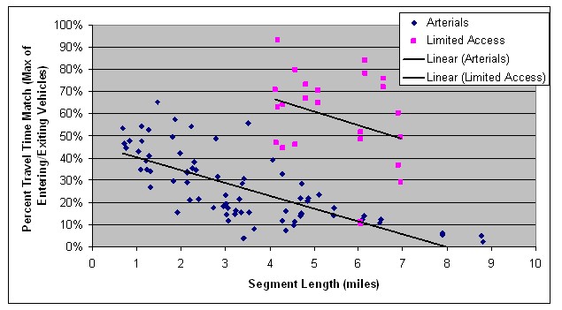
Figure 47. Tag Matching Efficiency versus Segment Length

4.7. Latency and Travel Time Estimation

The travel times experienced by actual travelers are different from those measured by either loop detectors or toll tag readers.

• For an actual traveler, the travel time experienced while traversing a segment is related to the travel speeds for the vehicle at different times as it traverses the segment.
• For loop detectors, travel time estimates are based on speed measurements made along the length of a segment at a particular point in time.
• For toll tag readers, the travel time estimates are based on the travel time experienced by travelers traversing a segment, but the measurement is delayed by the time required to complete the segment.

During times when travel times are relatively stable, all of these values will be similar. When travel times are changing, such as when congestion is building, these times can be different.

Consider what would occur for a segment where the usual travel time was 10 minutes after a crash occurred that instantly changed the travel time experienced by travelers to 30 minutes by introducing a 20-minute delay for those vehicle passing through the crash location. With loop detectors,⁶ the observed speeds would quickly change from pre-crash to post-crash values, and the travel time estimated using loop detectors would change quickly from 10 minutes to 30 minutes.

For toll tag readers, the result would be different. During the first few minutes after the crash, vehicles already downstream of the crash location would continue to arrive at the end of the travel time segment and the system would continue to measure 10-minute travel times. After that, there would be a period during which few vehicles arrived at the end of the travel time segment because the vehicles were caught in the delay caused by the crash. The system might note that fewer vehicles were arriving than expected, but would have no travel time data to indicate that travel times had increased. After 30 minutes had passed, those vehicles delayed by the crash would arrive at the end of the travel time segment and the system would report 30 minute travel times.

Toll tag readers introduce a delay in producing travel time estimates equal to the estimated travel time.

Thus, travel times estimates produced by loop detectors respond quickly to changes in travel times that may occur. Travel time estimates produced by toll tag readers are delayed by the time required for the vehicles that enter the travel time segment to completely traverse the segment - the estimates are delayed by a time equal to the travel time estimate. While this delay is modest for short travel time segments, it can be long for longer travel time segments. For example, the iFlorida arterial toll tag reader deployment included a number of travel time segments that were 5 miles or more in length. Travel time along these segments during congested periods could exceed 30 minutes, which meant that the estimated travel times reflected travel times experienced by travelers entering the segment 30 minutes earlier rather than current traffic conditions. Thus, although toll tag readers produce accurate travel time estimates, in that they reflect travel times experienced by actual travelers, the delay in obtaining the estimate can limit the usefulness of the resulting estimates.

The latency inherent in toll tag based traffic monitoring systems could limit its effectiveness for incident detection.

This latency inherent in toll tag based traffic monitoring systems can also impact the usefulness of toll tag reader networks for incident detection. In order for automated incident detection to be useful, an incident should be identified within minutes of when it occurred. Because the measurement delay in a toll tag based traffic monitoring system is equal to the travel time for the segment, this type of system would provide effective incident detection only if the toll tag readers were spaced sufficiently close so that the expected travel time was less than time delay allowed for effective incident detection.

4.8. Summary and Conclusions

As part of the iFlorida Model Deployment, FDOT deployed a network of toll tag readers that were used to estimate travel times on seven Orlando arterials and on portions of several limited access toll roads. Soon after the deployment of these readers was complete in May 2005, FDOT discovered that many of them had failed between the time they were deployed and FDOT began monitoring them. From that time until early in 2006, FDOT struggled to achieve reliable operations with these readers. The reader network operated reliably for the first six months of 2006, though configuration problems with the CRS software made it uncertain whether the travel times being produced by this network were being used correctly to provide 511 travel time messages. Beginning in May 2006, the operational reliability of the toll tag network dropped again. Stable operations were restored in January 2007 and continued through June 2007, when the reliability dropped again as FDOT transitioned from the warranty period, where the deployment vendor was responsible for most repair activities, to a period where FDOT was responsible for maintenance. The CRS software also failed in June 2007, and it was not until November 2007 that FDOT had procured new software that would ingest travel times from the toll tag network and automatically populate 511 messages with those travel times.

Throughout this process, lessons learned regarding the operation of a toll tag network for estimating travel times were documented. These lessons learned are summarized in the following list, with more details provided in the preceeding sections of this report.

• FDOT identified and/or experienced a number of factors that limited the effectiveness of the toll tag network for producing travel times. Those considering using toll tag based travel time networks should consider these factors in their designs. Some of the factors FDOT identified and problems they experienced included:
  • Limited market penetration for toll tag readers. Before deploying a toll tag network, FDOT conducted tests indicating that about 20 percent of vehicles on Orlando arterials had toll tag readers, indicating that toll tag readers would generate a large number of reads for the iFlorida arterials.
  • Misaligned toll tag readers. After deployment, FDOT found that some toll tag readers did not produce as many reads as expected. FDOT discovered misaligned antennae and obstructions between the antennae and the roadway were often the root cause of this problem.
  • Duplicate tag reads. On arterials, vehicles often passed under the toll tag readers at low speeds or were stopped under the reader. This often resulted in duplicate reads of the same tag.
  • Vehicle diversions. FDOT found that many tags read at the start of a travel time segment did not match any tags read exiting the segment. This was likely caused by vehicles diverting onto other roads before exiting the segment. The fraction of vehicles diverting seemed to increase as the travel time segment length increased.
  • Vehicle stops. An analysis of travel time observations indicated that the mean observed travel time was typically significantly higher than the median observed travel time. This was likely because some vehicles made stops between the time they entered and exited a travel time segment, introducing a high bias into the travel time observations. Methods were needed to filter out these high travel time outliers.
  • Toll tag reader failures. FDOT experienced a large number of reader failures early in the deployment and struggled to maintain high availability of the readers throughout the project. At peak performance, about 90 percent of readers were operational, though the percent of operational readers could be much lower.
  • Clock mis-synchronization. When first deployed, the internal clocks on many of the toll tag readers were not synchronized with a standard clock, which prevented use of the toll tag reader data for computing travel times.
  • Transmission of archived tag reads. The FDOT toll tag reader system maintained an archive of toll tags read at each reader. If the transmission the tag information to the toll tag server failed, the reader would later re-transmit all of the tag reads that had previously failed to transmit. At times, this transmission required so much network bandwidth that the transmission of real-time toll tag reads from other readers was delayed, which prevented the use of the real-time data to generate real-time travel time esimates.
• Travel time estimation parameters. The algorithm that FDOT used to generate travel times from the toll tag reader data was originally developed for use on limited access highways. FDOT discovered that some of the parameter settings needed to be different to work well on arterials. For example, diverting traffic on arterials meant that the observed average travel time was typically higher than the actual travel time, which was not the case on limited access highways. The algorithm for excluding outliers is, therefore, more important on arterials than for limited access highways.
• Including tag reads from turning vehicles can increase the number of travel time observations generated. The FDOT algorithms used data from a single reader to supply tag reads for both the entrance into and exit from a travel time segment. Depending on the exact placement of the readers relative to the intersection, more matches can be obtained by allowing data from multiple readers to be used. (For example, if a reader supplying tag reads at the entrance of a travel time segment is placed upstream the starting intersection, then it will not record tag reads from turning vehicles that enter the segment. Including tag reads from readers monitoring the intersecting road can provide reads from these turning vehicles.) The evaluation team tested such an algorithm and found a significant increase in the number of travel time observations recorded.
• Toll tag reader monitoring should began as soon as deployment is complete. The iFlorida toll tag readers were deployed over a four month period, and FDOT did not begin actively monitoring the reader status until the deployment was complete. In the intervening period, many readers had failed, which created a large demand for reader repairs that FDOT was not able to fulfill.
• Downstream systems should include methods to continue operations when reader failures occur. Even when operating well, about ten percent of iFlorida toll tag readers were out of service. Yet, the CRS methods for handling missing data from toll tag readers were not very robust - in most cases, the data was simply treated as missing. An approach to fill in the missing data with estimates from historical data or operator observations would have helped FDOT continue to provide complete traveler information services even when toll tag readers failed.
• The toll tag matching efficiency was much higher for limited access roads than for arterials and much lower for long arterials than for short ones. For short aterial segments (about 1 mile in length), about 50 percent of entering vehicles were later observed exiting the segment. For long arterial segments (about 5 miles in length), this percentage dropped to less than 20 percent.
• Using toll tag readers to estimate travel times introduces a delay in generating observed travel times—if a travel time of T minutes is observed, then that travel time applies to a vehicle that entered the segment T minutes ago. During times of rapid change in the segment travel time, this delay can reduce the usefulness of the travel time data. In particular, this delay may mean that toll tag readers are ineffective tools for incident detection.

---

¹ See the report Innovative Traffic Data Collection: Results of Field Test - Final Report prepared for FDOT on February 12, 2003 for more information.

² See the report Field Test of the Potential for Using Probe Vehicles to Determine Arterial Travel Times in the Orlando Metropolitan Area - Final Report prepared for FDOT on July 1, 2003 for more information.

³ These figures include matches that resulted in very long travel time estimates, likely resulting from vehicles that made stops or other diversions between two toll tag readers used to make a travel time estimate. A production travel time calculation tool would filter out these outliers, resulting in lower percentage for matching toll tag reads.

⁴ This data is available at http://www.dot.state.fl.us/planning/statistics/trafficdata/ accessed March 10, 2009.

⁵ More information on the challenges faced in deploying the toll tag reader network is contained in the report titled iFlorida Model Deployment-Deployment Experience Study completed in May 2006.

⁶ The system response would depend on the location of the loop detectors relative to the congestion. If no loops were located in the congested area, then the system would not detect the additional delay. If loops were concentrated in the congested area, the system might over-estimate the delay. This statement assumes that loops were placed so as to accurately measure the crash-induced delay.