Comprehensive Truck Size and Weight Limits Study - Bridge Structure Comparative Analysis Technical Report
Chapter 2: Structural Analysis and Bridge Posting Assessment
2.1 Overview
A total of 490 bridges out of a pool of more than 500 candidates were selected for inclusion into the final sample database representing the inventory of bridges on the National Highway System (NHS). The breakdown of this database was determined primarily based on the distribution of the bridge types on the NHS. Bridge selection was further refined to include additional considerations including year built, maximum span length, and live load capacity to get a diverse sample space. The breakdown of the bridges in the sample database is given in Table 1.
| Bridge Type | IS | Other NHS | TOTAL | ||||
|---|---|---|---|---|---|---|---|
| # of Bridges | Frequency (%) | # of Bridges | Frequency (%) | # of Bridges | Frequency (%) |
||
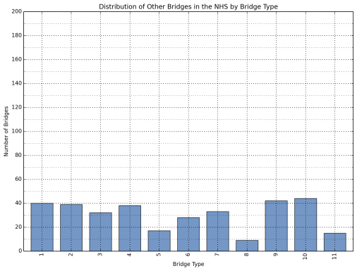
| 1 | Reinforced Concrete Slab | 18 | 11.8 | 40 | 11.9 | 58 | 11.8 |
| 2 | Pre-stressed Concrete Beam/Girder Simple Span | 30 | 19.6 | 39 | 11.6 | 69 | 14.1 |
| 3 | Pre-stressed Concrete Beam/Girder Continuous Span | 16 | 10.5 | 32 | 9.5 | 48 | 9.8 |
| 4 | Steel Beam/Girder Simple Span (L < 100 ft.) | 14 | 9.2 | 38 | 11.3 | 52 | 10.6 |
| 5 | Steel Beam/Girder, Simple Span (L >= 100 ft.) | 19 | 12.4 | 17 | 5.0 | 36 | 7.3 |
| 6 | Steel Beam/Girder, Continuous Spans (L < 100 ft.) | 21 | 13.7 | 28 | 8.3 | 49 | 10.0 |
| 7 | Steel Beam/Girder, Continuous Spans (L >= 100 ft.) | 11 | 7.2 | 33 | 9.8 | 44 | 9.0 |
| 8 | Girder Floor-beam Systems | 2 | 1.3 | 9 | 2.7 | 11 | 2.2 |
| 9 | Reinforced Concrete Tee Beam | 11 | 7.2 | 42 | 12.5 | 53 | 10.8 |
| 10 | Box Beams | 10 | 6.5 | 44 | 13.1 | 54 | 11.0 |
| 11 | Through Truss | 1 | 0.7 | 15 | 4.5 | 16 | 3.3 |
| TOTAL | 153 | 100.0 | 337 | 100.0 | 490 | 100.0 | |
Per the overarching project assumptions stated in the Volume II: Modal Shift Comparative Analysis, with the exception of the triple trailer combinations, the study parameters assume the scenario vehicles are able to travel wherever the control vehicles could operate. For analytical purposes triple trailer combinations (Scenarios 5 and 6) are assumed to be restricted to a 74,500 mile network of Interstate and other principal arterial highways. The structural analyses assessed in this study take into account the findings related to changes in vehicle use patterns that the study team projected would result from the availability of alternative vehicle configurations.
The AASHTOWare Bridge Rating® (ABrR) program was used to analyze the 490 bridges for the base case, (GVW ≤ 80,000 lbs. compared to GVW > 80,000 lbs.) and for the proposed alternate vehicles (alternate scenario, GVW >80,000 lb.). The load and resistance factor rating (LRFR) methodology was employed in the analysis for all bridge types, except girder-floor-beam systems and through trusses, where the load factor rating (LFR) method was used, since the ABrR software does not currently support LRFR methodology for these two bridge types.
Rating factors were extracted for alternative truck configurations and 3-S2 and 2-S1-2 control vehicles for both flexure and shear, and the results were investigated statistically. For each bridge type, the number of bridges having a rating factor less than 1.0 was extracted for all alternative truck configurations. This was performed for Interstate bridges and for other bridges on the NHS, separately. Next, the percentage of bridges that have posting issues for each bridge type, by each truck, was calculated by dividing the number of bridges with a RF less than 1.0 by the total number of bridges of that bridge type in the sample database.
In order to project the number of bridges that may need posting in the entire NHS inventory, the actual number of bridges in the NHS inventory for each bridge type was determined. The projected number of bridges to be posted in each category was calculated by multiplying the percentage of posted bridges in the sample database for a given bridge type by the actual number of bridges of the same type in the NHS inventory. Summary results from this statistical projection are given in Table 2.
| NUMBER OF BRIDGES IN THE NBI | LOAD RATING RESULTS | PROJECTED NUMBER OF BRIDGES W/ POSTING ISSUES FOR ENTIRE INVENTORY | ||||||
|---|---|---|---|---|---|---|---|---|
| # of IS Bridges in the NBI | # of Other NHS Bridges in the NBI | # of IS Bridges Rated | # of Other NHS Bridges Rated | Vehicle Configuration | IS Bridges Rated w/ RF < 1.0 (%) |
Other NHS Bridges Rated w/ RF < 1.0 (%) |
# of IS Bridges w/ Posting Issues | # of Other NHS Bridges w/ Posting Issues |
| 45417 | 43528 | 153 | 337 | Scenario 1 | 3.3% | 5.0% | 1485 | 2194 |
| Scenario 2 | 3.3% | 7.7% | 1485 | 3360 | ||||
| Scenario 3 | 4.6% | 9.5% | 2080 | 4135 | ||||
| Scenario 4 | 2.6% | 3.0% | 1185 | 1293 | ||||
| Scenario 5 | 2.0% | 0.9% | 890 | 387 | ||||
| Scenario 6 | 6.5% | 5.6% | 2970 | 2455 | ||||
The table above shows both the percentages and the actual number of bridges that have posting issues.
In order to estimate the probable one-time cost effect of employing alternative truck configurations, a methodology was developed and presented in this report. It estimates the increase in cost relative to the base vehicles. An RF of 1.0 was set as the acceptance criteria when determining bridge improvement needs. It should be noted the one-time cost of bridge improvements addressed herein could pertain to either superstructure strengthening or superstructure replacement triggered by the need to increase live load capacity. The choice of strengthening vs. replacement would depend on superstructure type and whichever is the more economical alternative.
2.2 Bridge Inventory Used In the Structural Analysis
Introduction
The diversity of the bridge infrastructure in terms of age and design parameters (including structural type, materials of construction, width, length, etc.) is broad. Experience has shown the performance of any specific bridge is dependent on complex interactions of multiple factors, many of which are closely linked and include the following: original design parameters and specifications, bridge type, materials of construction, geometry, design load, and incidence of corrosion or other deterioration processes.
The sample database of bridges was developed to gain a diverse representation of the bridges that make up the NHS inventory, which are broken down by type in Table 3. The bridge types in this table were determined based on the material of construction, distinct structural behavior, and span configurations (L denotes the longest span length).
| Bridge Type | IS | Other NHS | TOTAL | ||||
|---|---|---|---|---|---|---|---|
| # of Bridges | Frequency (%) | # of Bridges | Frequency (%) | # of Bridges | Frequency (%) |
||
| 1 | Reinforced Concrete Slab | 5101 | 11.2% | 4903 | 11.2% | 10004 | 11.2% |
| 2 | Pre-stressed Concrete Beam/Girder Simple Span | 9382 | 20.6% | 11079 | 25.4% | 20461 | 23.0% |
| 3 | Pre-stressed Concrete Beam/Girder Continuous Span | 2131 | 4.7% | 3817 | 8.8% | 5948 | 6.8% |
| 4 | Steel Beam/Girder Simple Span (L < 100 ft.) | 6183 | 13.6% | 5195 | 11.9% | 11378 | 12.8% |
| 5 | Steel Beam/Girder, Simple Span (L > = 100 ft.) | 2847 | 6.3% | 1983 | 4.6% | 4830 | 5.4% |
| 6 | Steel Beam/Girder, Continuous Spans (L < 100 ft.) | 6755 | 14.9% | 3958 | 9.1% | 10713 | 12.0% |
| 7 | Steel Beam/Girder, Continuous Spans (L > = 100 ft.) | 4255 | 9.4% | 3158 | 7.3% | 7413 | 8.3% |
| 8 | Girder Floor-beam Systems | 774 | 1.7% | 553 | 1.3% | 1327 | 1.5% |
| 9 | Reinforced Concrete Tee Beam | 2639 | 5.8% | 3499 | 8.0% | 6138 | 6.9% |
| 10 | Box Beams | 5248 | 11.6% | 5094 | 11.7% | 10342 | 11.6% |
| 11 | Through Truss | 102 | 0.2% | 289 | 0.7% | 391 | 0.5% |
| TOTAL | 45,417 | 100% | 43,528 | 100% | 88,945 | 100% | |
A total of 490 bridges were selected for the sample database representing the NHS inventory. In order to verify whether the number of bridges in the sample database is adequate, the study team used Slovin’s formula:
![]()
Where:
N = the number of bridges in the total population
e = the margin of error
n = the required number of bridges in the sample database (which corresponds to the confidence level per the margin of error provided).
For a 95 percent confidence level, the required number of bridges in the sample database can be calculated as:
![]()
Thus, it can be stated that by using 490 bridges in the sample database, a confidence level of more than 95 percent was achieved. The exact confidence level of the sample database can be computed by rewriting the Slovin’s formula as:
![]()
![]()
The breakdown of the sample database was determined primarily based on the distribution of bridge types in the NHS inventory. Bridge selection was further refined to include additional considerations including year built, maximum span length, and live load capacity to get a diverse sample space. The breakdown of the final sample database of bridges used in this study is shown in Table 4.
| Bridge Type | IS | Other NHS | TOTAL | ||||
|---|---|---|---|---|---|---|---|
| # of Bridges | Frequency (%) | # of Bridges | Frequency (%) | # of Bridges | Frequency (%) |
||
| 1 | Reinforced Concrete Slab | 18 | 11.8 | 40 | 11.9 | 58 | 11.8 |
| 2 | Pre-stressed Concrete Beam/Girder Simple Span | 30 | 19.6 | 39 | 11.6 | 69 | 14.1 |
| 3 | Pre-stressed Concrete Beam/Girder Continuous Span | 16 | 10.5 | 32 | 9.5 | 48 | 9.8 |
| 4 | Steel Beam/Girder Simple Span (L < 100 ft.) | 14 | 9.2 | 38 | 11.3 | 52 | 10.6 |
| 5 | Steel Beam/Girder, Simple Span (L >= 100 ft.) | 19 | 12.4 | 17 | 5.0 | 36 | 7.3 |
| 6 | Steel Beam/Girder, Continuous Spans (L < 100 ft.) | 21 | 13.7 | 28 | 8.3 | 49 | 10.0 |
| 7 | Steel Beam/Girder, Continuous Spans (L >= 100 ft.) | 11 | 7.2 | 33 | 9.8 | 44 | 9.0 |
| 8 | Girder Floor-beam Systems | 2 | 1.3 | 9 | 2.7 | 11 | 2.2 |
| 9 | Reinforced Concrete Tee Beam | 11 | 7.2 | 42 | 12.5 | 53 | 10.8 |
| 10 | Box Beams | 10 | 6.5 | 44 | 13.1 | 54 | 11.0 |
| 11 | Through Truss | 1 | 0.7 | 15 | 4.5 | 16 | 3.3 |
| TOTAL | 153 | 100.0 | 337 | 100.0 | 490 | 100.0 | |
Bridges were selected from all regions of the country. The sample database consists of bridges from 11 States as shown in Table 5. Span lengths and age of construction of these bridges are also described in the tables and plots to follow.
| States | # of Bridges | Frequency (%) |
|---|---|---|
| Illinois | 96 | 19.6 |
| New York | 103 | 21.0 |
| Virginia | 23 | 4.7 |
| Michigan | 66 | 13.5 |
| Louisiana | 20 | 4.1 |
| New Mexico | 34 | 6.9 |
| Utah | 74 | 15.1 |
| S. Dakota | 14 | 2.9 |
| Alabama | 33 | 6.7 |
| New Jersey | 23 | 4.7 |
| Idaho | 4 | 0.8 |
| TOTAL | 490 | 100.0 |
The distribution of the bridges in the sample database is shown in Figure 1 through Figure 3 for all bridges, Interstate bridges, and other bridges on the NHS, respectively.
Figure 1: Distribution of All Bridges by Bridge Type.
(See Table 3 for description of bridge types)
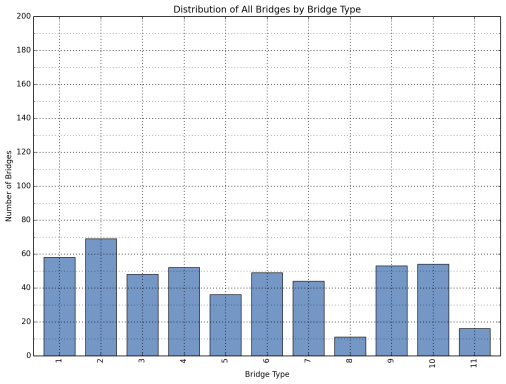
Figure 2: Distribution of Interstate Bridges by Bridge Type.
(See Table 3 for description of bridge types)
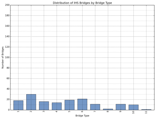
Figure 3: Distribution of Other Bridges on the NHS by Bridge Type.
(See Table 3 for description of bridge types)
Distribution of Bridges by Span Length
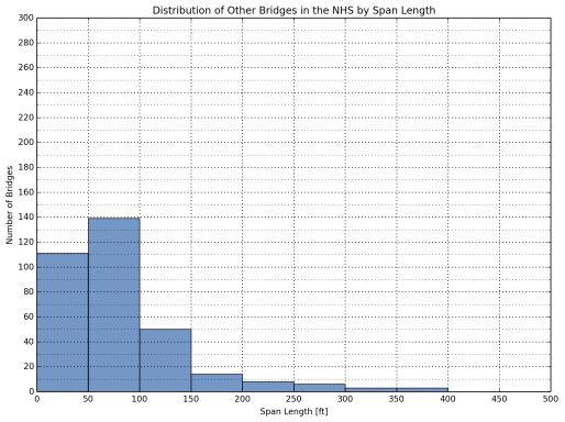
The distribution of the bridges in the sample database by span length is listed in Table 6. The bulk of the bridges analyzed in this study have a span length less than or equal to 150 ft. (91.4 percent for Interstate and other NHS bridges combined). Span length distributions are illustrated in Figure 4 through Figure 6 for all bridges, Interstate bridges, and other bridges on the NHS, respectively.
| Span Length | IS | Other NHS | TOTAL | |||
|---|---|---|---|---|---|---|
| # of Bridges | Frequency (%) |
# of Bridges | Frequency (%) |
# of Bridges | Frequency (%) |
|
| <50 | 35 | 21.6 | 111 | 33.8 | 146 | 29.8 |
| 50-100 | 77 | 47.5 | 136 | 41.5 | 213 | 43.5 |
| 100-150 | 33 | 20.4 | 56 | 17.1 | 89 | 18.2 |
| 150-200 | 7 | 4.3 | 10 | 3.0 | 17 | 3.5 |
| 200-250 | 4 | 2.5 | 4 | 1.2 | 8 | 1.6 |
| 250-300 | 2 | 1.2 | 6 | 1.8 | 8 | 1.6 |
| 300-350 | 0 | 0.0 | 2 | 0.6 | 2 | 0.4 |
| 350-400 | 1 | 0.6 | 2 | 0.6 | 3 | 0.6 |
| 400-450 | 0 | 0.0 | 0 | 0.0 | 0 | 0.0 |
| 450-500 | 1 | 0.6 | 0 | 0.0 | 1 | 0.2 |
| >500 | 2 | 1.2 | 1 | 0.3 | 3 | 0.6 |
| TOTAL | 162 | 100.0 | 328 | 100.0 | 490 | 100.0 |
Figure 4: Distribution of All Bridges by Span Length
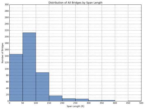
Figure 5: Distribution of Interstate Bridges by Span Length
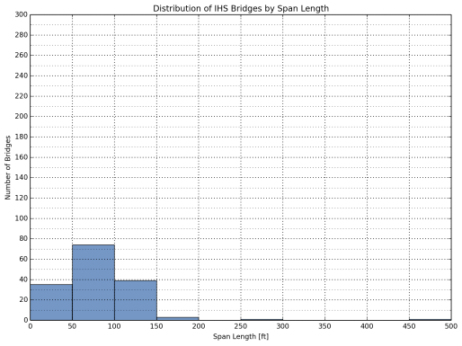
Figure 6: Distribution of Other Bridges on the NHS by Span Length
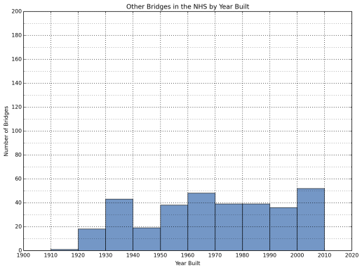
Distribution of Bridges by Year Built
The distribution of the bridges in the sample database by year built is listed in Table 7. Those designated “other NHS bridges” have an approximately uniform distribution between 1920 and 2010. On the other hand, almost no Interstate bridges were recorded before the time interval 1950-1960, and bulk of the Interstate bridges (74.5 percent) analyzed in this study were built between 1950 and 1980. This is due to the fact that the Interstate System was built when President Dwight D. Eisenhower signed the Federal-Aid Highway Act of 1956.
| Span Length | IS | Other NHS | TOTAL | |||
|---|---|---|---|---|---|---|
| # of Bridges | Frequency (%) |
# of Bridges | Frequency (%) |
# of Bridges | Frequency (%) |
|
| <=1920 | 0 | 0.0 | 2 | 0.6 | 2 | 0.4 |
| 1920-1930 | 0 | 0.0 | 20 | 5.9 | 20 | 4.1 |
| 1930-1940 | 0 | 0.0 | 42 | 12.5 | 42 | 8.6 |
| 1940-1950 | 0 | 0.0 | 21 | 6.2 | 21 | 4.3 |
| 1950-1960 | 21 | 13.7 | 41 | 12.2 | 62 | 12.7 |
| 1960-1970 | 58 | 37.9 | 45 | 13.4 | 103 | 21.0 |
| 1970-1980 | 35 | 22.9 | 37 | 11.0 | 72 | 14.7 |
| 1980-1990 | 18 | 11.8 | 38 | 11.3 | 56 | 11.4 |
| 1990-2000 | 11 | 7.2 | 40 | 11.9 | 51 | 10.4 |
| >2000 | 10 | 6.5 | 51 | 15.1 | 61 | 12.4 |
| TOTAL | 153 | 100.0 | 337 | 100.0 | 490 | 100.0 |
Figure 7: Distribution of All Bridges by Built Year
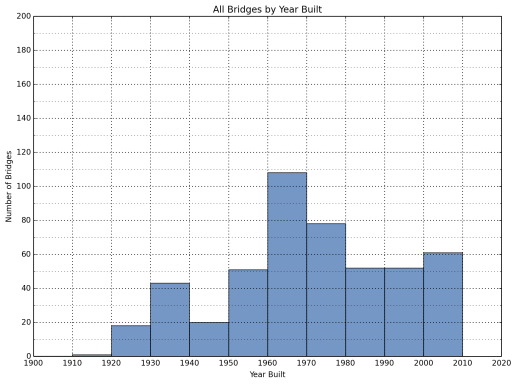
Figure 8: Distribution of Interstate Bridges by Built Year
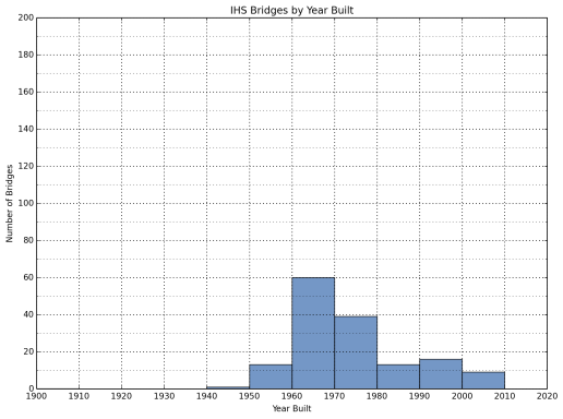
Figure 9: Distribution of Other Bridges on the NHS by Built Year
2.3 Load Rating Results For All Bridges
Load Rating Results for All Bridge Types (Raw Rating Factors)
Non-normalized rating factors from each truck are given in Table 8 and Table 9 for flexural and shear rating factors, respectively. Table 8 and Table 9 also include the maximum and minimum rating factors observed in the sample database as well as the number of bridges with a rating factor (RF) less than 1.0, which would require load posting.
Average rating factors for each truck are also illustrated in Figure 10 and Figure 11 for flexure and shear ratings, respectively. These figures show that flexure tends to yield lower rating factors compared to shear. In other words, in most of the bridges in the sample database, load ratings were controlled by flexure. Consistently higher average rating factors were observed for Interstate bridges compared to other bridges on the NHS, although the difference was not found to be very significant. On average, the first group of vehicles (3-S2 and Scenarios 1, 2 and 3) resulted in lower rating factors compared to the second group (2-S1-2 and Scenarios 4, 5 and 6). When the study team investigated trucks within vehicle groups, Scenario 3 and Scenario 6 yielded the lowest rating factors in the first and second group, respectively.
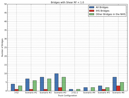
Lastly, the number of bridges with an RF less than 1.0, which would require posting, is shown in Figure 12 for the flexural case and Figure 13 for the shear case.
| 3-S2 | Scenario #1 | Scenario #2 | Scenario #3 | 2-S1-2 | Scenario #4 | Scenario #5 | Scenario #6 | ||
|---|---|---|---|---|---|---|---|---|---|
| ALL BRIDGES | AVERAGE | 3.816 | 3.442 | 3.228 | 2.984 | 4.591 | 3.862 | 4.094 | 3.133 |
| MAX | 19.86 | 18.06 | 17.38 | 16.06 | 28.07 | 22.55 | 26.26 | 20.10 | |
| MIN | 0.707 | 0.626 | 0.591 | 0.541 | 0.806 | 0.728 | 0.660 | 0.516 | |
| TOTAL | 463 | 463 | 463 | 463 | 463 | 463 | 463 | 463 | |
| # RF < 1.0 | 4 | 7 | 8 | 10 | 1 | 2 | 3 | 8 | |
| IHS BRIDGES | AVERAGE | 3.679 | 3.319 | 3.106 | 2.876 | 4.330 | 3.697 | 3.806 | 2.911 |
| MAX | 13.58 | 12.27 | 11.73 | 10.99 | 15.40 | 13.70 | 13.12 | 9.35 | |
| MIN | 0.997 | 0.896 | 0.837 | 0.781 | 1.136 | 1.014 | 0.922 | 0.723 | |
| TOTAL | 150 | 150 | 150 | 150 | 150 | 150 | 150 | 150 | |
| # RF < 1.0 | 1 | 1 | 1 | 2 | 0 | 0 | 1 | 3 | |
| OTHER BRIDGES ON THE NHS | AVERAGE | 3.881 | 3.501 | 3.286 | 3.036 | 4.715 | 3.941 | 4.232 | 3.240 |
| MAX | 19.86 | 18.06 | 17.38 | 16.06 | 28.07 | 22.55 | 26.26 | 20.10 | |
| MIN | 0.707 | 0.626 | 0.591 | 0.541 | 0.806 | 0.728 | 0.660 | 0.516 | |
| TOTAL | 313 | 313 | 313 | 313 | 313 | 313 | 313 | 313 | |
| # RF < 1.0 | 3 | 6 | 7 | 8 | 1 | 2 | 2 | 5 | |
Figure 10: Comparison of Average Flexural Rating Factors for Different Truck Types
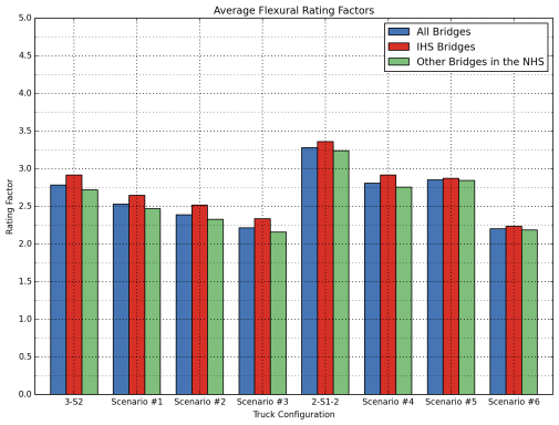
Figure 11: Comparison of Average Shear Rating Factors for Different Truck Types
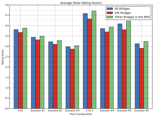
Figure 12: Comparison of Number of Bridges that Require Posting Due to Flexure for Different Truck Types
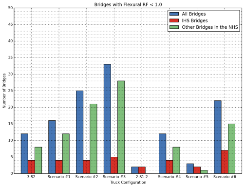
Figure 13: Comparison of Number of Bridges that Require Posting Due to Shear for Different Truck Types
Comparisons of Baseline Trucks with Other Vehicles
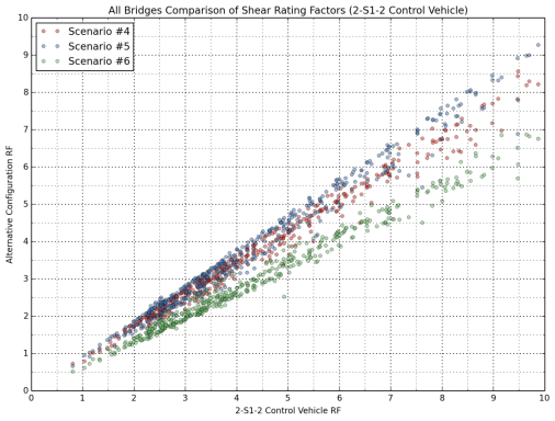
Scatter plots were constructed to investigate the comparative rating results from the control vehicles (3-S2 and 2-S1-2) and the alternative truck configurations, where the 3-S2 control vehicle was compared with Scenarios 1, 2 and 3, and the 2-S1-2 control vehicle was compared with Scenarios 4, 5 and 6. These comparisons are shown in Figure 14 through Figure 17 for all bridges in the sample database. Separate comparisons for Interstate bridges and other bridges on the NHS are provided in Appendix C.
When the 3-S2 control vehicle was compared to alternate truck configuration (Scenarios 1, 2 and 3), a linear correlation was observed in both flexural (Figure 14) and shear (Figure 16) ratings between the control vehicle and the other three scenarios, but more scatter was observed in shear ratings.
Comparisons of the 2-S1-2 control vehicle and Scenarios 4, 5 and 6 show more scatter compared to the first group of trucks (3-S2 and, Scenarios 1, 2 and 3) for both flexure (Figure 15) and shear (Figure 17), and this effect is much more pronounced in the shear ratings.
Figure 14: Comparison of Flexural Rating Factors for All Bridges (Compared with 3-S2)
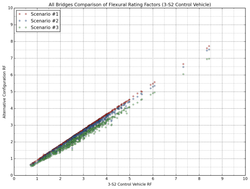
Figure 15: Comparison of Flexural Rating Factors for All Bridges (Compared with 2-S1-2)
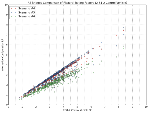
Figure 16: Comparison of Shear Rating Factors for All Bridges (Compared with 3-S2)
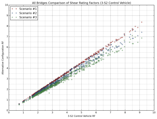
Figure 17: Comparison of Shear Rating Factors for All Bridges (Compared with 2-S1-2)
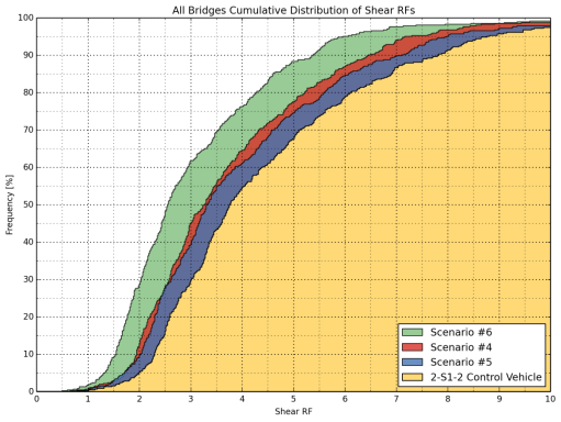
Cumulative Frequency Distribution Functions for Rating Results
Cumulative frequency distribution functions are helpful in visually determining the percentage of bridges falling below a given rating factor. The cumulative distribution functions for each truck group were constructed for both flexure and shear cases, as shown in Figure 18 through Figure 21 for all bridges in the sample database. Separate comparisons for Interstate bridges and other bridges in the NHS are provided in the bridge appendix.
It was observed that Scenarios 1, 2, and 3 result in consistently lower flexure and shear ratings than the 3-S2 control vehicle, where Scenario 1 yields the highest and Scenario 3 yields the lowest RF among the three while Scenario 2 yields RFs in between (Figure 18 and Figure 20).
When the 2-S1-2 control vehicle and Scenarios 4, 5, and 6 configurations were compared, similarly to the first group of trucks, it was seen that Scenarios 4, 5 and 6 would result in lower ratings compared to the control vehicle. The configuration with the lowest RFs was found to be Scenario 6. An overlap was observed for Scenarios 4 and 5 when the flexural case was considered, meaning that these scenario vehicles generally yield similar results (Figure 19 and Figure 21).
Figure 18: Cumulative Distribution of Flexural Rating Factors of All Bridges
(3-S2, Scenarios 1-3)
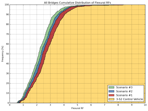
Figure 19: Cumulative Distribution of Flexural Rating Factors of All Bridges
(2-S1-2, Scenarios 4-6)
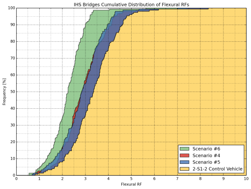
Figure 20: Cumulative Distribution of Shear Rating Factors of All Bridges
(3-S2, Scenarios 1-3)
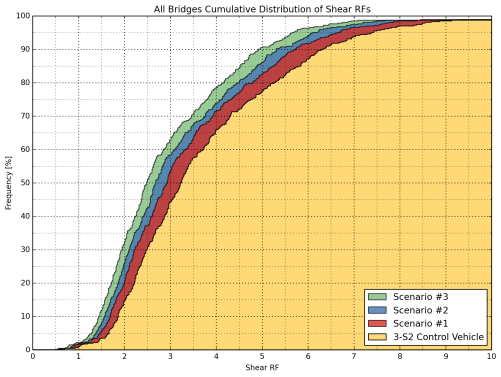
Figure 21: Cumulative Distribution of Shear Rating Factors of All Bridges
(2-S1-2, Scenarios 4-6)
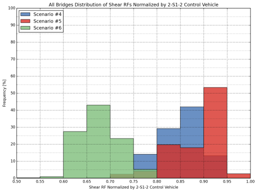
Load Rating Results for All Bridge Types (Normalized Rating Factors)
The following tables and plots present the normalized load rating results for all bridge types. The normalization was performed by divided the RFs computed for Scenarios 1, 2, and 3 by the RF calculated for the 3-S2 control vehicle. A similar normalization was performed for Scenarios 4, 5, and 6, where the RFs calculated for these configurations were dividing by the RF computed for the 2-S1-2 control vehicle. Tables include the average, maximum and minimum values, as well as the coefficient of variation (COV), which is a measure of relative dispersion in the results. A distribution of normalized RFs for each truck group were constructed for both flexure and shear cases, as shown in Figure 22 through Figure 25 for all bridges in the sample database. Separate comparisons for Interstate bridges and other bridges in the NHS are provided in Appendix C.
| NORMALIZED BY 3-S2 | NORMALIZED BY 2-S1-2 | ||||||
|---|---|---|---|---|---|---|---|
| Scenario 1 | Scenario 2 | Scenario 3 | Scenario 4 | Scenario 5 | Scenario 6 | ||
| ALL BRIDGES | AVERAGE | 0.907 | 0.851 | 0.790 | 0.854 | 0.868 | 0.674 |
| MAX | 0.976 | 1.075 | 1.008 | 1.045 | 0.964 | 0.874 | |
| MIN | 0.725 | 0.652 | 0.605 | 0.530 | 0.512 | 0.387 | |
| COV (%) | 1.2 | 5.1 | 5.3 | 7.0 | 8.8 | 8.3 | |
| IS BRIDGES | AVERAGE | 0.907 | 0.851 | 0.789 | 0.856 | 0.864 | 0.676 |
| MAX | 0.976 | 0.986 | 0.911 | 1.045 | 0.944 | 0.802 | |
| MIN | 0.884 | 0.743 | 0.686 | 0.695 | 0.572 | 0.465 | |
| COV (%) | 0.9 | 4.7 | 4.9 | 7.3 | 8.8 | 8.2 | |
| OTHER BRIDGES ON THE NHS | AVERAGE | 0.907 | 0.851 | 0.790 | 0.853 | 0.871 | 0.674 |
| MAX | 0.923 | 1.075 | 1.008 | 0.956 | 0.964 | 0.874 | |
| MIN | 0.725 | 0.652 | 0.605 | 0.530 | 0.512 | 0.387 | |
| COV (%) | 1.3 | 5.3 | 5.5 | 6.9 | 8.8 | 8.3 | |
Note: GFB systems and trusses not included.
| NORMALIZED BY 3-S2 | NORMALIZED BY 2-S1-2 | ||||||
|---|---|---|---|---|---|---|---|
| Scenario 1 | Scenario 2 | Scenario 3 | Scenario 4 | Scenario 5 | Scenario 6 | ||
| ALL BRIDGES | AVERAGE | 0.901 | 0.846 | 0.782 | 0.848 | 0.882 | 0.678 |
| MAX | 0.924 | 1.075 | 1.008 | 0.912 | 0.986 | 0.844 | |
| MIN | 0.789 | 0.719 | 0.596 | 0.688 | 0.699 | 0.512 | |
| COV (%) | 1.3 | 4.1 | 4.3 | 5.4 | 6.6 | 6.4 | |
| IS BRIDGES | AVERAGE | 0.900 | 0.843 | 0.779 | 0.849 | 0.877 | 0.676 |
| MAX | 0.924 | 0.986 | 0.911 | 0.912 | 0.954 | 0.799 | |
| MIN | 0.789 | 0.719 | 0.596 | 0.726 | 0.717 | 0.512 | |
| COV (%) | 1.6 | 3.9 | 4.2 | 5.7 | 6.4 | 7.2 | |
| OTHER BRIDGES ON THE NHS | AVERAGE | 0.902 | 0.847 | 0.784 | 0.847 | 0.885 | 0.679 |
| MAX | 0.922 | 1.075 | 1.008 | 0.909 | 0.986 | 0.844 | |
| MIN | 0.868 | 0.770 | 0.706 | 0.688 | 0.699 | 0.575 | |
| COV (%) | 1.2 | 4.2 | 4.4 | 5.2 | 6.8 | 6.0 | |
Note: GFB systems and trusses not included.
Figure 22: Distribution of Normalized Flexural Rating Factors for All Bridges
(3-S2, Scenario 1, 2 and 3)
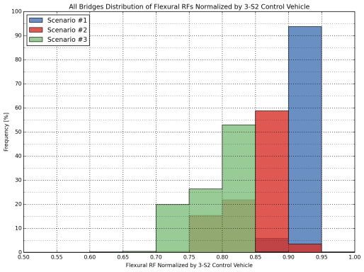
Figure 23: Distribution of Normalized Flexural Rating Factors for All Bridges
(2-S1-2, Scenario 4, 5 and 6)
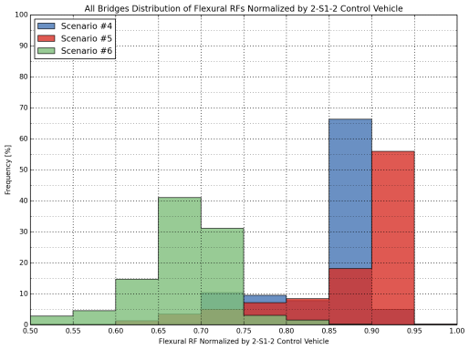
Figure 24: Distribution of Normalized Shear Rating Factors for All Bridges
(3-S2, Scenario 1, 2 And 3)
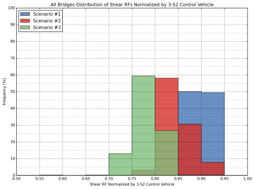
Figure 25: Distribution of Normalized Shear Rating Factors for All Bridges
(2-S1-2, Scenario 4, 5 and 6)
Load Rating Results for Bridge Types
Detailed load rating results based on raw rating factors and normalized rating factors for each bridge type analyzed in this study are tabulated in Appendix C of this report.
2.4 Posting Analysis
Summary
In order to investigate the effect of using alternate truck configurations on load posting, the sample database was filtered for bridges with rating factors less than 1.0. Secondly, the filtered database was sorted primarily by bridge type, and also by span length and by built year.
In 2011, the FHWA National Bridge Inventory included 43,528 bridges on the National Highway System (NHS); 45,417 of these bridges are located on the Interstate System. In 2014, 1,242 bridges that were posted on the NHS with 236 of these posted bridges located on the Interstate System. These posting are based on data reported to FHWA by the states in their submission of annual National Bridge Inventory data. It should be noted, criteria and policies applied to the posting of bridges varies from state to state. Analysis in this area of the Study focused on estimating the number of bridges that would be posted associated with each of the scenarios assessed. The costs to strengthen or replace bridges unable to accommodate scenario vehicles were also estimated. Based on the derived rating factors for each of the alternative truck configurations in each scenario, an assessment was made on the number of bridges that had posting issues and would potentially require either strengthening or replacement. A threshold Rating Factor (RF) value of 1.0 establishes a potential need for bridge strengthening or replacement. Table 12 shows the projected number of posted bridges associated with each scenario assessed in the Study.
For each bridge type, the number of bridges having a rating factor less than 1.0 was extracted for all alternate configurations (Scenarios 1 to 6). This was performed for Interstate bridges and for other bridges on the NHS, separately. Next, the percentage of bridges that need to be posted for each bridge type, by each truck, was calculated by dividing the number of bridges with a RF less than 1.0 by the total number of bridges in that category in the sample database. Resulting percentages are given in Table 13.
In order to project the number of bridges that may need posting in the entire NHS inventory, the actual number of bridges in the NHS inventory for each bridge type was determined. The projected number of bridges to be posted in each category was calculated by multiplying the percentage of posted bridges in the sample database for a given bridge type (computed in Table 13) by the actual number of bridges of the same type in the NHS inventory. The projected number of bridges on the NHS inventory that may require load posting is given in detail in Table 14, separately for Interstate bridges and for other bridges on the NHS, for each vehicle type. Summary results are listed in Table 12.
| NUMBER OF BRIDGES IN THE NBI | LOAD RATING RESULTS | PROJECTED NUMBER OF BRIDGES W/ POSTING ISSUES FOR ENTIRE INVENTORY | ||||||
|---|---|---|---|---|---|---|---|---|
| # of IS Bridges in the NBI | # of Other NHS Bridges in the NBI | # of IS Bridges Rated | # of Other NHS Bridges Rated | Vehicle Configuration | IS Bridges Rated w/ RF < 1.0 (%) |
Other NHS Bridges Rated w/ RF < 1.0 (%) |
# of IS Bridges w/ Posting Issues | # of Other NHS Bridges w/ Posting Issues |
| 45417 | 43528 | 153 | 337 | Scenario 1 | 3.3% | 5.0% | 1485 | 2194 |
| Scenario 2 | 3.3% | 7.7% | 1485 | 3360 | ||||
| Scenario 3 | 4.6% | 9.5% | 2080 | 4135 | ||||
| Scenario 4 | 2.6% | 3.0% | 1185 | 1293 | ||||
| Scenario 5 | 2.0% | 0.9% | 890 | 387 | ||||
| Scenario 6 | 6.5% | 5.6% | 2970 | 2455 | ||||
The effect of the alternative truck configurations on the rating results is more pronounced in the “other NHS bridges” category (Highway Network 2) due to the larger sample space.
In addition, the filtered database of bridges with RFs less than 1.0 was sorted by span lengths, using 20 ft. increments, as listed in Table 15. The percentage of bridges that need to be posted for each span length interval was calculated in a similar manner to that which was performed for bridge types.
Lastly, the filtered database of bridges with RFs less than 1.0 was sorted by year built, using 10 year intervals, as listed in Table 16. The percentage of bridges that need to be posted for each 10 year interval was calculated in a similar manner to that which was performed for bridge types.
| Bridge Type | #. of IHS Bridges Rated | # of Other NHS Bridges Rated | Vehicle Configuration | RF < 1.0 Flexure Controls |
RF < 1.0 Shear Controls |
Flex or Shear RF < 1.0 | # of IHS Bridges w/ RF < 1.0 | # of Other NHS Bridges w/ RF < 1.0 | % of IHS Bridges Rated w/ RF < 1.0 | % of Other NHS Bridges Rated w/ RF < 1.0 | |
|---|---|---|---|---|---|---|---|---|---|---|---|
| 1 | Concrete Slab | 18 | 40 | 3-S2 | 4 | 0 | 4 | 2 | 2 | 11.1% | 5.0% |
| 18 | 40 | Scenario #1 | 5 | 0 | 5 | 2 | 3 | 11.1% | 7.5% | ||
| 18 | 40 | Scenario #2 | 8 | 0 | 8 | 2 | 6 | 11.1% | 15.0% | ||
| 18 | 40 | Scenario #3 | 10 | 0 | 10 | 2 | 8 | 11.1% | 20.0% | ||
| 18 | 40 | 2-S1-2 | 0 | 0 | 0 | 0 | 0 | 0.0% | 0.0% | ||
| 18 | 40 | Scenario #4 | 3 | 0 | 3 | 2 | 1 | 11.1% | 2.5% | ||
| 18 | 40 | Scenario #5 | 0 | 0 | 0 | 0 | 0 | 0.0% | 0.0% | ||
| 18 | 40 | Scenario #6 | 4 | 0 | 4 | 2 | 2 | 11.1% | 5.0% | ||
| 2 | Concrete Girder / Simple span | 30 | 39 | 3-S2 | 1 | 0 | 1 | 1 | 0 | 3.3% | 0.0% |
| 30 | 39 | Scenario #1 | 1 | 0 | 1 | 1 | 0 | 3.3% | 0.0% | ||
| 30 | 39 | Scenario #2 | 1 | 0 | 1 | 1 | 0 | 3.3% | 0.0% | ||
| 30 | 39 | Scenario #3 | 2 | 0 | 2 | 2 | 0 | 6.7% | 0.0% | ||
| 30 | 39 | 2-S1-2 | 1 | 0 | 1 | 1 | 0 | 3.3% | 0.0% | ||
| 30 | 39 | Scenario #4 | 1 | 0 | 1 | 1 | 0 | 3.3% | 0.0% | ||
| 30 | 39 | Scenario #5 | 1 | 0 | 1 | 1 | 0 | 3.3% | 0.0% | ||
| 30 | 39 | Scenario #6 | 2 | 0 | 2 | 2 | 0 | 6.7% | 0.0% | ||
| 3 | Concrete Girder / Cont. spans | 16 | 32 | 3-S2 | 1 | 0 | 1 | 1 | 0 | 6.3% | 0.0% |
| 16 | 32 | Scenario #1 | 1 | 0 | 1 | 1 | 0 | 6.3% | 0.0% | ||
| 16 | 32 | Scenario #2 | 2 | 0 | 2 | 1 | 1 | 6.3% | 3.1% | ||
| 16 | 32 | Scenario #3 | 2 | 0 | 2 | 1 | 1 | 6.3% | 3.1% | ||
| 16 | 32 | 2-S1-2 | 1 | 0 | 1 | 1 | 0 | 6.3% | 0.0% | ||
| 16 | 32 | Scenario #4 | 2 | 0 | 2 | 1 | 1 | 6.3% | 3.1% | ||
| 16 | 32 | Scenario #5 | 2 | 0 | 2 | 1 | 1 | 6.3% | 3.1% | ||
| 16 | 32 | Scenario #6 | 2 | 1 | 3 | 2 | 1 | 12.5% | 3.1% | ||
| 4 | Steel Girder / Simple span, L < 100 | 14 | 38 | 3-S2 | 2 | 0 | 2 | 0 | 2 | 0.0% | 5.3% |
| 14 | 38 | Scenario #1 | 2 | 0 | 2 | 0 | 2 | 0.0% | 5.3% | ||
| 14 | 38 | Scenario #2 | 4 | 0 | 4 | 0 | 4 | 0.0% | 10.5% | ||
| 14 | 38 | Scenario #3 | 4 | 0 | 4 | 0 | 4 | 0.0% | 10.5% | ||
| 14 | 38 | 2-S1-2 | 0 | 0 | 0 | 0 | 0 | 0.0% | 0.0% | ||
| 14 | 38 | Scenario #4 | 2 | 0 | 2 | 0 | 2 | 0.0% | 5.3% | ||
| 14 | 38 | Scenario #5 | 0 | 0 | 0 | 0 | 0 | 0.0% | 0.0% | ||
| 14 | 38 | Scenario #6 | 2 | 0 | 2 | 0 | 2 | 0.0% | 5.3% | ||
| 5 | Steel Girder / Simple span, L > 100 | 19 | 17 | 3-S2 | 0 | 2 | 2 | 1 | 1 | 5.3% | 5.9% |
| 19 | 17 | Scenario #1 | 0 | 2 | 2 | 1 | 1 | 5.3% | 5.9% | ||
| 19 | 17 | Scenario #2 | 0 | 2 | 2 | 1 | 1 | 5.3% | 5.9% | ||
| 19 | 17 | Scenario #3 | 0 | 2 | 2 | 1 | 1 | 5.3% | 5.9% | ||
| 19 | 17 | 2-S1-2 | 0 | 1 | 1 | 0 | 1 | 0.0% | 5.9% | ||
| 19 | 17 | Scenario #4 | 0 | 1 | 1 | 0 | 1 | 0.0% | 5.9% | ||
| 19 | 17 | Scenario #5 | 0 | 2 | 2 | 1 | 1 | 5.3% | 5.9% | ||
| 19 | 17 | Scenario #6 | 2 | 2 | 4 | 2 | 2 | 10.5% | 11.8% | ||
| 6 | Steel Girder / Cont. spans, L < 100 | 21 | 28 | 3-S2 | 0 | 0 | 0 | 0 | 0 | 0.0% | 0.0% |
| 21 | 28 | Scenario #1 | 0 | 0 | 0 | 0 | 0 | 0.0% | 0.0% | ||
| 21 | 28 | Scenario #2 | 0 | 0 | 0 | 0 | 0 | 0.0% | 0.0% | ||
| 21 | 28 | Scenario #3 | 1 | 0 | 1 | 0 | 1 | 0.0% | 3.6% | ||
| 21 | 28 | 2-S1-2 | 0 | 0 | 0 | 0 | 0 | 0.0% | 0.0% | ||
| 21 | 28 | Scenario #4 | 0 | 0 | 0 | 0 | 0 | 0.0% | 0.0% | ||
| 21 | 28 | Scenario #5 | 0 | 0 | 0 | 0 | 0 | 0.0% | 0.0% | ||
| 21 | 28 | Scenario #6 | 1 | 0 | 1 | 0 | 1 | 0.0% | 3.6% | ||
| 7 | Steel Girder / Cont. spans, L > 100 | 11 | 33 | 3-S2 | 0 | 0 | 0 | 0 | 0 | 0.0% | 0.0% |
| 11 | 33 | Scenario #1 | 0 | 0 | 0 | 0 | 0 | 0.0% | 0.0% | ||
| 11 | 33 | Scenario #2 | 0 | 0 | 0 | 0 | 0 | 0.0% | 0.0% | ||
| 11 | 33 | Scenario #3 | 0 | 0 | 0 | 0 | 0 | 0.0% | 0.0% | ||
| 11 | 33 | 2-S1-2 | 0 | 0 | 0 | 0 | 0 | 0.0% | 0.0% | ||
| 11 | 33 | Scenario #4 | 0 | 0 | 0 | 0 | 0 | 0.0% | 0.0% | ||
| 11 | 33 | Scenario #5 | 0 | 0 | 0 | 0 | 0 | 0.0% | 0.0% | ||
| 11 | 33 | Scenario #6 | 1 | 0 | 1 | 1 | 0 | 9.1% | 0.0% | ||
| 8 | Steel Girder / Floor-beam * | 2 | 9 | 3-S2 | N/A | N/A | 0 | 0 | 0 | 0.0% | 0.0% |
| 2 | 9 | Scenario #1 | N/A | N/A | 0 | 0 | 0 | 0.0% | 0.0% | ||
| 2 | 9 | Scenario #2 | N/A | N/A | 0 | 0 | 0 | 0.0% | 0.0% | ||
| 2 | 9 | Scenario #3 | N/A | N/A | 0 | 0 | 0 | 0.0% | 0.0% | ||
| 2 | 9 | 2-S1-2 | N/A | N/A | 0 | 0 | 0 | 0.0% | 0.0% | ||
| 2 | 9 | Scenario #4 | N/A | N/A | 0 | 0 | 0 | 0.0% | 0.0% | ||
| 2 | 9 | Scenario #5 | N/A | N/A | 0 | 0 | 0 | 0.0% | 0.0% | ||
| 2 | 9 | Scenario #6 | N/A | N/A | 0 | 0 | 0 | 0.0% | 0.0% | ||
| 9 | Conc. Tee beams | 11 | 42 | 3-S2 | 4 | 2 | 6 | 0 | 6 | 0.0% | 14.3% |
| 11 | 42 | Scenario #1 | 7 | 4 | 11 | 0 | 11 | 0.0% | 26.2% | ||
| 11 | 42 | Scenario #2 | 9 | 5 | 14 | 0 | 14 | 0.0% | 33.3% | ||
| 11 | 42 | Scenario #3 | 11 | 6 | 17 | 1 | 16 | 9.1% | 38.1% | ||
| 11 | 42 | 2-S1-2 | 0 | 0 | 0 | 0 | 0 | 0.0% | 0.0% | ||
| 11 | 42 | Scenario #4 | 4 | 1 | 5 | 0 | 5 | 0.0% | 11.9% | ||
| 11 | 42 | Scenario #5 | 0 | 1 | 1 | 0 | 1 | 0.0% | 2.4% | ||
| 11 | 42 | Scenario #6 | 7 | 5 | 12 | 1 | 11 | 9.1% | 26.2% | ||
| 10 | Conc. Box beams | 10 | 44 | 3-S2 | 0 | 0 | 0 | 0 | 0 | 0.0% | 0.0% |
| 10 | 44 | Scenario #1 | 0 | 0 | 0 | 0 | 0 | 0.0% | 0.0% | ||
| 10 | 44 | Scenario #2 | 0 | 0 | 0 | 0 | 0 | 0.0% | 0.0% | ||
| 10 | 44 | Scenario #3 | 1 | 0 | 1 | 0 | 1 | 0.0% | 2.3% | ||
| 10 | 44 | 2-S1-2 | 0 | 0 | 0 | 0 | 0 | 0.0% | 0.0% | ||
| 10 | 44 | Scenario #4 | 0 | 0 | 0 | 0 | 0 | 0.0% | 0.0% | ||
| 10 | 44 | Scenario #5 | 0 | 0 | 0 | 0 | 0 | 0.0% | 0.0% | ||
| 10 | 44 | Scenario #6 | 0 | 0 | 0 | 0 | 0 | 0.0% | 0.0% | ||
| 11 | Steel Through truss* | 1 | 15 | 3-S2 | Axial | Axial | 0 | 0 | 0 | 0.0% | 0.0% |
| 1 | 15 | Scenario #1 | Axial | Axial | 0 | 0 | 0 | 0.0% | 0.0% | ||
| 1 | 15 | Scenario #2 | Axial | Axial | 0 | 0 | 0 | 0.0% | 0.0% | ||
| 1 | 15 | Scenario #3 | Axial | Axial | 0 | 0 | 0 | 0.0% | 0.0% | ||
| 1 | 15 | 2-S1-2 | Axial | Axial | 0 | 0 | 0 | 0.0% | 0.0% | ||
| 1 | 15 | Scenario #4 | Axial | Axial | 0 | 0 | 0 | 0.0% | 0.0% | ||
| 1 | 15 | Scenario #5 | Axial | Axial | 0 | 0 | 0 | 0.0% | 0.0% | ||
| 1 | 15 | Scenario #6 | Axial | Axial | 0 | 0 | 0 | 0.0% | 0.0% | ||
| TOTAL | 153 | 337 | 3-S2 | 16 | 5 | 11 | 3.3% | 3.3% | |||
| 153 | 337 | Scenario #1 | 22 | 5 | 17 | 3.3% | 5.0% | ||||
| 153 | 337 | Scenario #2 | 31 | 5 | 26 | 3.3% | 7.7% | ||||
| 153 | 337 | Scenario #3 | 39 | 7 | 32 | 4.6% | 9.5% | ||||
| 153 | 337 | 2-S1-2 | 3 | 2 | 1 | 1.3% | 0.3% | ||||
| 153 | 337 | Scenario #4 | 14 | 4 | 10 | 2.6% | 3.0% | ||||
| 153 | 337 | Scenario #5 | 6 | 3 | 3 | 2.0% | 0.9% | ||||
| 153 | 337 | Scenario #6 | 29 | 10 | 19 | 6.5% | 5.6% | ||||
N/A: Not applicable.
*: Girder-floor-beam systems and through trusses were rated using the Load Factor Rating (LFR) methodology. All other bridge types were rated using the Load and Resistance Factor Rating (LRFR) methodology.
| LOAD RATING RESULTS | PROJECTED NUMBER OF BRIDGES WITH POSTING ISSUES FOR ENTIRE INVENTORY | |||||||
|---|---|---|---|---|---|---|---|---|
| Bridge Type | #. of IHS Bridges Rated | # of Other NHS Bridges Rated | Vehicle Configuration | % of IHS Bridges Rated w/ RF < 1.0 | % of Other NHS Bridges Rated w/ RF < 1.0 | #. of IHS Bridges with Posting Issues | # of Other NHS Bridges with Posting Issues | |
| 1 | Concrete Slab | 18 | 40 | Scenario #1 | 11.1% | 7.5% | 566 | 368 |
| 18 | 40 | Scenario #2 | 11.1% | 15.0% | 566 | 735 | ||
| 18 | 40 | Scenario #3 | 11.1% | 20.0% | 566 | 981 | ||
| 18 | 40 | Scenario #4 | 11.1% | 2.5% | 566 | 123 | ||
| 18 | 40 | Scenario #5 | 0.0% | 0.0% | 0 | 0 | ||
| 18 | 40 | Scenario #6 | 11.1% | 5.0% | 566 | 245 | ||
| 2 | Concrete Girder / Simple span | 30 | 39 | Scenario #1 | 3.3% | 0.0% | 310 | 0 |
| 30 | 39 | Scenario #2 | 3.3% | 0.0% | 310 | 0 | ||
| 30 | 39 | Scenario #3 | 6.7% | 0.0% | 629 | 0 | ||
| 30 | 39 | Scenario #4 | 3.3% | 0.0% | 310 | 0 | ||
| 30 | 39 | Scenario #5 | 3.3% | 0.0% | 310 | 0 | ||
| 30 | 39 | Scenario #6 | 6.7% | 0.0% | 629 | 0 | ||
| 3 | Concrete Girder / Cont. spans | 16 | 32 | Scenario #1 | 6.3% | 0.0% | 134 | 0 |
| 16 | 32 | Scenario #2 | 6.3% | 3.1% | 134 | 118 | ||
| 16 | 32 | Scenario #3 | 6.3% | 3.1% | 134 | 118 | ||
| 16 | 32 | Scenario #4 | 6.3% | 3.1% | 134 | 118 | ||
| 16 | 32 | Scenario #5 | 6.3% | 3.1% | 134 | 118 | ||
| 16 | 32 | Scenario #6 | 12.5% | 3.1% | 266 | 118 | ||
| 4 | Steel Girder / Simple span, L < 100 |
14 | 38 | Scenario #1 | 0.0% | 5.3% | 0 | 275 |
| 14 | 38 | Scenario #2 | 0.0% | 10.5% | 0 | 545 | ||
| 14 | 38 | Scenario #3 | 0.0% | 10.5% | 0 | 545 | ||
| 14 | 38 | Scenario #4 | 0.0% | 5.3% | 0 | 275 | ||
| 14 | 38 | Scenario #5 | 0.0% | 0.0% | 0 | 0 | ||
| 14 | 38 | Scenario #6 | 0.0% | 5.3% | 0 | 275 | ||
| 5 | Steel Girder / Simple span, L > 100 | 19 | 17 | Scenario #1 | 5.3% | 5.9% | 151 | 117 |
| 19 | 17 | Scenario #2 | 5.3% | 5.9% | 151 | 117 | ||
| 19 | 17 | Scenario #3 | 5.3% | 5.9% | 151 | 117 | ||
| 19 | 17 | Scenario #4 | 0.0% | 5.9% | 0 | 117 | ||
| 19 | 17 | Scenario #5 | 5.3% | 5.9% | 151 | 117 | ||
| 19 | 17 | Scenario #6 | 10.5% | 11.8% | 299 | 234 | ||
| 6 | Steel Girder / Cont. spans, L < 100 | 21 | 28 | Scenario #1 | 0.0% | 0.0% | 0 | 0 |
| 21 | 28 | Scenario #2 | 0.0% | 0.0% | 0 | 0 | ||
| 21 | 28 | Scenario #3 | 0.0% | 3.6% | 0 | 142 | ||
| 21 | 28 | Scenario #4 | 0.0% | 0.0% | 0 | 0 | ||
| 21 | 28 | Scenario #5 | 0.0% | 0.0% | 0 | 0 | ||
| 21 | 28 | Scenario #6 | 0.0% | 3.6% | 0 | 142 | ||
| 7 | Steel Girder / Cont. spans, L > 100 | 11 | 33 | Scenario #1 | 0.0% | 0.0% | 0 | 0 |
| 11 | 33 | Scenario #2 | 0.0% | 0.0% | 0 | 0 | ||
| 11 | 33 | Scenario #3 | 0.0% | 0.0% | 0 | 0 | ||
| 11 | 33 | Scenario #4 | 0.0% | 0.0% | 0 | 0 | ||
| 11 | 33 | Scenario #5 | 0.0% | 0.0% | 0 | 0 | ||
| 11 | 33 | Scenario #6 | 9.1% | 0.0% | 387 | 0 | ||
| 8 | Steel Girder / Floorbeam* | 2 | 9 | Scenario #1 | 0.0% | 0.0% | 0 | 0 |
| 2 | 9 | Scenario #2 | 0.0% | 0.0% | 0 | 0 | ||
| 2 | 9 | Scenario #3 | 0.0% | 0.0% | 0 | 0 | ||
| 2 | 9 | Scenario #4 | 0.0% | 0.0% | 0 | 0 | ||
| 2 | 9 | Scenario #5 | 0.0% | 0.0% | 0 | 0 | ||
| 2 | 9 | Scenario #6 | 0.0% | 0.0% | 0 | 0 | ||
| 9 | Conc. Tee beams | 11 | 42 | Scenario #1 | 0.0% | 26.2% | 0 | 917 |
| 11 | 42 | Scenario #2 | 0.0% | 33.3% | 0 | 1165 | ||
| 11 | 42 | Scenario #3 | 9.1% | 38.1% | 240 | 1333 | ||
| 11 | 42 | Scenario #4 | 0.0% | 11.9% | 0 | 416 | ||
| 11 | 42 | Scenario #5 | 0.0% | 2.4% | 0 | 84 | ||
| 11 | 42 | Scenario #6 | 9.1% | 26.2% | 240 | 917 | ||
| 10 | Conc. Box beams | 10 | 44 | Scenario #1 | 0.0% | 0.0% | 0 | 0 |
| 10 | 44 | Scenario #2 | 0.0% | 0.0% | 0 | 0 | ||
| 10 | 44 | Scenario #3 | 0.0% | 2.3% | 0 | 117 | ||
| 10 | 44 | Scenario #4 | 0.0% | 0.0% | 0 | 0 | ||
| 10 | 44 | Scenario #5 | 0.0% | 0.0% | 0 | 0 | ||
| 10 | 44 | Scenario #6 | 0.0% | 0.0% | 0 | 0 | ||
| 11 | Steel Through Truss* | 1 | 15 | Scenario #1 | 0.0% | 0.0% | 0 | 0 |
| 1 | 15 | Scenario #2 | 0.0% | 0.0% | 0 | 0 | ||
| 1 | 15 | Scenario #3 | 0.0% | 0.0% | 0 | 0 | ||
| 1 | 15 | Scenario #4 | 0.0% | 0.0% | 0 | 0 | ||
| 1 | 15 | Scenario #5 | 0.0% | 0.0% | 0 | 0 | ||
| 1 | 15 | Scenario #6 | 0.0% | 0.0% | 0 | 0 | ||
| TOTAL | 153 | 337 | Scenario #1 | 3.3% | 5.0% | 1485 | 2194 | |
| 153 | 337 | Scenario #2 | 3.3% | 7.7% | 1485 | 3360 | ||
| 153 | 337 | Scenario #3 | 4.6% | 9.5% | 2080 | 4135 | ||
| 153 | 337 | Scenario #4 | 2.6% | 3.0% | 1185 | 1293 | ||
| 153 | 337 | Scenario #5 | 2.0% | 0.9% | 890 | 387 | ||
| 153 | 337 | Scenario #6 | 6.5% | 5.6% | 2970 | 2455 | ||
*: Girder-floor-beam systems and through trusses were rated using the Load Factor Rating (LFR) methodology. All other bridge types were rated using the Load and Resistance Factor Rating (LRFR) methodology.
| Span Length [ft.] |
# of IHS Bridges Rated | # of Other NHS Bridges Rated | Vehicle Configuration | # of IHS Bridges w/ RF < 1.0 | # of Other NHS Bridges w/ RF < 1.0 | % of IHS Bridges Rated w/ RF < 1.0 | % of Other NHS Bridges Rated w/ RF < 1.0 |
|---|---|---|---|---|---|---|---|
| <20 | 0 | 8 | Scenario #1 | 0 | 0 | 0.0% | 0.0% |
| 0 | 8 | Scenario #2 | 0 | 1 | 0.0% | 12.5% | |
| 0 | 8 | Scenario #3 | 0 | 1 | 0.0% | 12.5% | |
| 0 | 8 | Scenario #4 | 0 | 0 | 0.0% | 0.0% | |
| 0 | 8 | Scenario #5 | 0 | 0 | 0.0% | 0.0% | |
| 0 | 8 | Scenario #6 | 0 | 0 | 0.0% | 0.0% | |
| 20-40 | 24 | 67 | Scenario #1 | 2 | 10 | 8.3% | 14.9% |
| 24 | 67 | Scenario #2 | 2 | 13 | 8.3% | 19.4% | |
| 24 | 67 | Scenario #3 | 2 | 16 | 8.3% | 23.9% | |
| 24 | 67 | Scenario #4 | 2 | 5 | 8.3% | 7.5% | |
| 24 | 67 | Scenario #5 | 0 | 0 | 0.0% | 0.0% | |
| 24 | 67 | Scenario #6 | 2 | 6 | 8.3% | 9.0% | |
| 40-60 | 25 | 76 | Scenario #1 | 1 | 5 | 4.0% | 6.6% |
| 25 | 76 | Scenario #2 | 1 | 8 | 4.0% | 10.5% | |
| 25 | 76 | Scenario #3 | 2 | 10 | 8.0% | 13.2% | |
| 25 | 76 | Scenario #4 | 1 | 2 | 4.0% | 2.6% | |
| 25 | 76 | Scenario #5 | 1 | 1 | 4.0% | 1.3% | |
| 25 | 76 | Scenario #6 | 1 | 7 | 4.0% | 9.2% | |
| 60-80 | 31 | 59 | Scenario #1 | 1 | 1 | 3.2% | 1.7% |
| 31 | 59 | Scenario #2 | 1 | 2 | 3.2% | 3.4% | |
| 31 | 59 | Scenario #3 | 2 | 2 | 6.5% | 3.4% | |
| 31 | 59 | Scenario #4 | 1 | 2 | 3.2% | 3.4% | |
| 31 | 59 | Scenario #5 | 1 | 1 | 3.2% | 1.7% | |
| 31 | 59 | Scenario #6 | 3 | 2 | 9.7% | 3.4% | |
| 80-100 | 31 | 44 | Scenario #1 | 0 | 0 | 0.0% | 0.0% |
| 31 | 44 | Scenario #2 | 0 | 1 | 0.0% | 2.3% | |
| 31 | 44 | Scenario #3 | 0 | 2 | 0.0% | 4.5% | |
| 31 | 44 | Scenario #4 | 0 | 0 | 0.0% | 0.0% | |
| 31 | 44 | Scenario #5 | 0 | 0 | 0.0% | 0.0% | |
| 31 | 44 | Scenario #6 | 1 | 2 | 3.2% | 4.5% | |
| 100-120 | 22 | 32 | Scenario #1 | 1 | 1 | 4.5% | 3.1% |
| 22 | 32 | Scenario #2 | 1 | 1 | 4.5% | 3.1% | |
| 22 | 32 | Scenario #3 | 1 | 1 | 4.5% | 3.1% | |
| 22 | 32 | Scenario #4 | 0 | 1 | 0.0% | 3.1% | |
| 22 | 32 | Scenario #5 | 1 | 1 | 4.5% | 3.1% | |
| 22 | 32 | Scenario #6 | 1 | 2 | 4.5% | 6.3% | |
| 120-140 | 14 | 11 | Scenario #1 | 0 | 0 | 0.0% | 0.0% |
| 14 | 11 | Scenario #2 | 0 | 0 | 0.0% | 0.0% | |
| 14 | 11 | Scenario #3 | 0 | 0 | 0.0% | 0.0% | |
| 14 | 11 | Scenario #4 | 0 | 0 | 0.0% | 0.0% | |
| 14 | 11 | Scenario #5 | 0 | 0 | 0.0% | 0.0% | |
| 14 | 11 | Scenario #6 | 0 | 0 | 0.0% | 0.0% | |
| 140-160 | 2 | 10 | Scenario #1 | 0 | 0 | 0.0% | 0.0% |
| 2 | 10 | Scenario #2 | 0 | 0 | 0.0% | 0.0% | |
| 2 | 10 | Scenario #3 | 0 | 0 | 0.0% | 0.0% | |
| 2 | 10 | Scenario #4 | 0 | 0 | 0.0% | 0.0% | |
| 2 | 10 | Scenario #5 | 0 | 0 | 0.0% | 0.0% | |
| 2 | 10 | Scenario #6 | 0 | 0 | 0.0% | 0.0% | |
| 160-180 | 1 | 6 | Scenario #1 | 0 | 0 | 0.0% | 0.0% |
| 1 | 6 | Scenario #2 | 0 | 0 | 0.0% | 0.0% | |
| 1 | 6 | Scenario #3 | 0 | 0 | 0.0% | 0.0% | |
| 1 | 6 | Scenario #4 | 0 | 0 | 0.0% | 0.0% | |
| 1 | 6 | Scenario #5 | 0 | 0 | 0.0% | 0.0% | |
| 1 | 6 | Scenario #6 | 1 | 0 | 100.0% | 0.0% | |
| 180-200 | 1 | 1 | Scenario #1 | 0 | 0 | 0.0% | 0.0% |
| 1 | 1 | Scenario #2 | 0 | 0 | 0.0% | 0.0% | |
| 1 | 1 | Scenario #3 | 0 | 0 | 0.0% | 0.0% | |
| 1 | 1 | Scenario #4 | 0 | 0 | 0.0% | 0.0% | |
| 1 | 1 | Scenario #5 | 0 | 0 | 0.0% | 0.0% | |
| 1 | 1 | Scenario #6 | 1 | 0 | 100.0% | 0.0% | |
| >200 | 2 | 23 | Scenario #1 | 0 | 0 | 0.0% | 0.0% |
| 2 | 23 | Scenario #2 | 0 | 0 | 0.0% | 0.0% | |
| 2 | 23 | Scenario #3 | 0 | 0 | 0.0% | 0.0% | |
| 2 | 23 | Scenario #4 | 0 | 0 | 0.0% | 0.0% | |
| 2 | 23 | Scenario #5 | 0 | 0 | 0.0% | 0.0% | |
| 2 | 23 | Scenario #6 | 0 | 0 | 0.0% | 0.0% | |
| TOTAL | 153 | 337 | Scenario #1 | 5 | 17 | 3.3% | 5.0% |
| 153 | 337 | Scenario #2 | 5 | 26 | 3.3% | 7.7% | |
| 153 | 337 | Scenario #3 | 7 | 32 | 4.6% | 9.5% | |
| 153 | 337 | Scenario #4 | 4 | 10 | 2.6% | 3.0% | |
| 153 | 337 | Scenario #5 | 3 | 3 | 2.0% | 0.9% | |
| 153 | 337 | Scenario #6 | 10 | 19 | 6.5% | 5.6% |
| Year Built | #. of IHS Bridges Rated | # of Other NHS Bridges Rated | Vehicle Configuration | # of IHS Bridges w/ RF < 1.0 | # of Other NHS Bridges w/ RF < 1.0 | % of IHS Bridges Rated w/ RF < 1.0 | % of Other NHS Bridges Rated w/ RF < 1.0 |
|---|---|---|---|---|---|---|---|
| <1920 | 0 | 2 | Scenario #1 | 0 | 0 | 0.0% | 0.0% |
| 0 | 2 | Scenario #2 | 0 | 1 | 0.0% | 50.0% | |
| 0 | 2 | Scenario #3 | 0 | 1 | 0.0% | 50.0% | |
| 0 | 2 | Scenario #4 | 0 | 0 | 0.0% | 0.0% | |
| 0 | 2 | Scenario #5 | 0 | 0 | 0.0% | 0.0% | |
| 0 | 2 | Scenario #6 | 0 | 0 | 0.0% | 0.0% | |
| 1920-1930 | 0 | 20 | Scenario #1 | 0 | 2 | 0.0% | 10.0% |
| 0 | 20 | Scenario #2 | 0 | 3 | 0.0% | 15.0% | |
| 0 | 20 | Scenario #3 | 0 | 4 | 0.0% | 20.0% | |
| 0 | 20 | Scenario #4 | 0 | 2 | 0.0% | 10.0% | |
| 0 | 20 | Scenario #5 | 0 | 0 | 0.0% | 0.0% | |
| 0 | 20 | Scenario #6 | 0 | 2 | 0.0% | 10.0% | |
| 1930-1940 | 0 | 42 | Scenario #1 | 0 | 6 | 0.0% | 14.3% |
| 0 | 42 | Scenario #2 | 0 | 9 | 0.0% | 21.4% | |
| 0 | 42 | Scenario #3 | 0 | 10 | 0.0% | 23.8% | |
| 0 | 42 | Scenario #4 | 0 | 3 | 0.0% | 7.1% | |
| 0 | 42 | Scenario #5 | 0 | 0 | 0.0% | 0.0% | |
| 0 | 42 | Scenario #6 | 0 | 6 | 0.0% | 14.3% | |
| 1940-1950 | 0 | 21 | Scenario #1 | 0 | 1 | 0.0% | 4.8% |
| 0 | 21 | Scenario #2 | 0 | 1 | 0.0% | 4.8% | |
| 0 | 21 | Scenario #3 | 0 | 3 | 0.0% | 14.3% | |
| 0 | 21 | Scenario #4 | 0 | 0 | 0.0% | 0.0% | |
| 0 | 21 | Scenario #5 | 0 | 0 | 0.0% | 0.0% | |
| 0 | 21 | Scenario #6 | 0 | 2 | 0.0% | 9.5% | |
| 1950-1960 | 21 | 41 | Scenario #1 | 0 | 2 | 0.0% | 4.9% |
| 21 | 41 | Scenario #2 | 0 | 5 | 0.0% | 12.2% | |
| 21 | 41 | Scenario #3 | 1 | 6 | 4.8% | 14.6% | |
| 21 | 41 | Scenario #4 | 0 | 1 | 0.0% | 2.4% | |
| 21 | 41 | Scenario #5 | 0 | 1 | 0.0% | 2.4% | |
| 21 | 41 | Scenario #6 | 1 | 4 | 4.8% | 9.8% | |
| 1960-1970 | 58 | 45 | Scenario #1 | 4 | 2 | 6.9% | 4.4% |
| 58 | 45 | Scenario #2 | 4 | 2 | 6.9% | 4.4% | |
| 58 | 45 | Scenario #3 | 4 | 2 | 6.9% | 4.4% | |
| 58 | 45 | Scenario #4 | 3 | 1 | 5.2% | 2.2% | |
| 58 | 45 | Scenario #5 | 2 | 1 | 3.4% | 2.2% | |
| 58 | 45 | Scenario #6 | 5 | 2 | 8.6% | 4.4% | |
| 1970-1980 | 35 | 37 | Scenario #1 | 0 | 1 | 0.0% | 0.0% |
| 35 | 37 | Scenario #2 | 0 | 1 | 0.0% | 0.0% | |
| 35 | 37 | Scenario #3 | 0 | 1 | 0.0% | 0.0% | |
| 35 | 37 | Scenario #4 | 0 | 0 | 0.0% | 0.0% | |
| 35 | 37 | Scenario #5 | 0 | 0 | 0.0% | 0.0% | |
| 35 | 37 | Scenario #6 | 0 | 0 | 0.0% | 0.0% | |
| 1980-1990 | 18 | 38 | Scenario #1 | 1 | 1 | 5.6% | 2.6% |
| 18 | 38 | Scenario #2 | 1 | 2 | 5.6% | 5.3% | |
| 18 | 38 | Scenario #3 | 2 | 3 | 11.1% | 7.9% | |
| 18 | 38 | Scenario #4 | 1 | 2 | 5.6% | 5.3% | |
| 18 | 38 | Scenario #5 | 1 | 1 | 5.6% | 2.6% | |
| 18 | 38 | Scenario #6 | 3 | 1 | 16.7% | 2.6% | |
| 1990-2000 | 11 | 40 | Scenario #1 | 0 | 2 | 0.0% | 5.0% |
| 11 | 40 | Scenario #2 | 0 | 2 | 0.0% | 5.0% | |
| 11 | 40 | Scenario #3 | 0 | 2 | 0.0% | 5.0% | |
| 11 | 40 | Scenario #4 | 0 | 1 | 0.0% | 2.5% | |
| 11 | 40 | Scenario #5 | 0 | 0 | 0.0% | 0.0% | |
| 11 | 40 | Scenario #6 | 0 | 2 | 0.0% | 5.0% | |
| >2000 | 10 | 51 | Scenario #1 | 0 | 0 | 0.0% | 0.0% |
| 10 | 51 | Scenario #2 | 0 | 0 | 0.0% | 0.0% | |
| 10 | 51 | Scenario #3 | 0 | 0 | 0.0% | 0.0% | |
| 10 | 51 | Scenario #4 | 0 | 0 | 0.0% | 0.0% | |
| 10 | 51 | Scenario #5 | 0 | 0 | 0.0% | 0.0% | |
| 10 | 51 | Scenario #6 | 1 | 0 | 10.0% | 0.0% | |
| TOTAL | 153 | 337 | Scenario #1 | 5 | 17 | 3.3% | 5.0% |
| 153 | 337 | Scenario #2 | 5 | 26 | 3.3% | 7.7% | |
| 153 | 337 | Scenario #3 | 7 | 32 | 4.6% | 9.5% | |
| 153 | 337 | Scenario #4 | 4 | 10 | 2.6% | 3.0% | |
| 153 | 337 | Scenario #5 | 3 | 3 | 2.0% | 0.9% | |
| 153 | 337 | Scenario #6 | 10 | 19 | 6.5% | 5.6% |
2.5 Load Effects Based On Span Lengths
In order to investigate the effect of live loads on the rating results, the USDOT study team computed moment and shear load effects for simple and continuous spans for span lengths from 20 ft. to 240 ft. Compared to the actual rating factors, where the resistance of members are also accounted for, this investigation is a more simplistic approach that isolates the live load parameter in the rating factor calculations. Note that load effects are not an indicator of the live load capacity or the safety of the structure under increasing truck weights, since they are not coupled with member resistances. Therefore, the RF comparisons presented earlier provide a more realistic assessment of the bridge performance under alternative truck configuration loads.
Table 17 and Table 18 list positive moments and shears for simple spans, whereas Table 19 lists negative moments for continuous spans. Load effects from the alternative truck configurations were also normalized by the related control vehicle for comparison purposes and listed in Table 20 to Table 22.
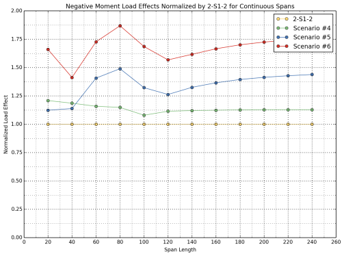
Load effects from Scenarios 1, 2, and 3 were normalized by load effects from 3-S2 control vehicle, and load effects from Scenarios 4, 5, and 6 were normalized by load effects from the 2-S1-2 control vehicle. Normalized load effects are also illustrated in Figure 26, Figure 28, and Figure 30 for the 3-S2 control vehicle as well as Scenarios 1, 2 and 3. Figure 27, Figure 29 and Figure 31 illustrate the normalized load effects for the 2-S1-2 control vehicle and Scenarios 4, 5, and 6.
| Span Length [ft.] |
3-S2 | Scenario 1 | Scenario 2 | Scenario 3 | 2-S1-2 | Scenario 4 | Scenario 5 | Scenario 6 |
|---|---|---|---|---|---|---|---|---|
| 20 | 136 | 151 | 170 | 184 | 85 | 121 | 96 | 115 |
| 40 | 329 | 363 | 406 | 440 | 228 | 291 | 248 | 352 |
| 60 | 559 | 612 | 643 | 696 | 470 | 534 | 514 | 710 |
| 80 | 790 | 862 | 904 | 976 | 800 | 892 | 865 | 1135 |
| 100 | 1147 | 1263 | 1297 | 1397 | 1153 | 1292 | 1301 | 1664 |
| 120 | 1530 | 1686 | 1733 | 1862 | 1506 | 1692 | 1799 | 2233 |
| 140 | 1914 | 2109 | 2170 | 2327 | 1859 | 2092 | 2327 | 2850 |
| 160 | 2311 | 2540 | 2607 | 2792 | 2212 | 2492 | 2854 | 3494 |
| 180 | 2710 | 2981 | 3044 | 3258 | 2565 | 2892 | 3382 | 4139 |
| 200 | 3110 | 3421 | 3491 | 3739 | 2918 | 3292 | 3909 | 4783 |
| 220 | 3509 | 3862 | 3946 | 4223 | 3271 | 3692 | 4437 | 5428 |
| 240 | 3909 | 4302 | 4401 | 4708 | 3624 | 4092 | 4964 | 6072 |
| Span Length [ft.] |
3-S2 | Scenario 1 | Scenario 2 | Scenario 3 | 2-S1-2 | Scenario 4 | Scenario 5 | Scenario 6 |
|---|---|---|---|---|---|---|---|---|
| 20 | 31 | 34 | 37 | 40 | 22 | 29 | 24 | 28 |
| 40 | 38 | 42 | 42 | 46 | 30 | 37 | 32 | 44 |
| 60 | 41 | 45 | 51 | 55 | 39 | 45 | 42 | 55 |
| 80 | 49 | 55 | 60 | 64 | 43 | 50 | 50 | 66 |
| 100 | 55 | 61 | 66 | 71 | 48 | 54 | 59 | 75 |
| 120 | 59 | 66 | 70 | 75 | 52 | 58 | 65 | 82 |
| 140 | 62 | 69 | 73 | 78 | 55 | 61 | 71 | 87 |
| 160 | 64 | 71 | 75 | 81 | 57 | 63 | 75 | 91 |
| 180 | 66 | 73 | 77 | 82 | 58 | 65 | 79 | 95 |
| 200 | 67 | 75 | 78 | 84 | 59 | 67 | 81 | 98 |
| 220 | 69 | 76 | 80 | 85 | 60 | 68 | 84 | 101 |
| 240 | 70 | 77 | 81 | 86 | 61 | 69 | 85 | 103 |
| Span Length [ft.] |
3-S2 | Scenario 1 | Scenario 2 | Scenario 3 | 2-S1-2 | Scenario 4 | Scenario 5 | Scenario 6 |
|---|---|---|---|---|---|---|---|---|
| 20 | -85 | -92 | -86 | -93 | -60 | -73 | -68 | -100 |
| 40 | -220 | -245 | -268 | -288 | -185 | -219 | -210 | -261 |
| 60 | -422 | -466 | -476 | -509 | -314 | -364 | -442 | -542 |
| 80 | -550 | -605 | -609 | -650 | -428 | -492 | -638 | -800 |
| 100 | -636 | -697 | -698 | -747 | -589 | -636 | -779 | -993 |
| 120 | -798 | -881 | -921 | -985 | -757 | -843 | -955 | -1186 |
| 140 | -988 | -1091 | -1135 | -1212 | -918 | -1028 | -1216 | -1484 |
| 160 | -1172 | -1294 | -1344 | -1434 | -1076 | -1209 | -1468 | -1792 |
| 180 | -1352 | -1492 | -1548 | -1651 | -1231 | -1385 | -1715 | -2091 |
| 200 | -1530 | -1687 | -1750 | -1865 | -1384 | -1560 | -1955 | -2385 |
| 220 | -1705 | -1881 | -1948 | -2076 | -1536 | -1732 | -2191 | -2674 |
| 240 | -1878 | -2072 | -2145 | -2286 | -1687 | -1904 | -2426 | -2960 |
| Span Length [ft.] |
NORMALIZED BY 3-S2 | NORMALIZED BY 2-S1-2 | ||||
|---|---|---|---|---|---|---|
| Scenario 1 | Scenario 2 | Scenario 3 | Scenario 4 | Scenario 5 | Scenario 6 | |
| 20 | 1.110 | 1.245 | 1.347 | 1.429 | 1.129 | 1.351 |
| 40 | 1.103 | 1.234 | 1.336 | 1.279 | 1.090 | 1.544 |
| 60 | 1.095 | 1.149 | 1.243 | 1.136 | 1.094 | 1.510 |
| 80 | 1.091 | 1.144 | 1.236 | 1.116 | 1.082 | 1.419 |
| 100 | 1.101 | 1.131 | 1.218 | 1.121 | 1.129 | 1.443 |
| 120 | 1.102 | 1.133 | 1.217 | 1.124 | 1.195 | 1.483 |
| 140 | 1.102 | 1.134 | 1.216 | 1.126 | 1.252 | 1.533 |
| 160 | 1.099 | 1.128 | 1.208 | 1.127 | 1.291 | 1.580 |
| 180 | 1.100 | 1.123 | 1.202 | 1.128 | 1.319 | 1.614 |
| 200 | 1.100 | 1.123 | 1.202 | 1.128 | 1.340 | 1.639 |
| 220 | 1.100 | 1.124 | 1.203 | 1.129 | 1.357 | 1.660 |
| 240 | 1.101 | 1.126 | 1.204 | 1.129 | 1.370 | 1.676 |
| Span Length [ft.] |
NORMALIZED BY 3-S2 | NORMALIZED BY 2-S1-2 | ||||
|---|---|---|---|---|---|---|
| Scenario 1 | Scenario 2 | Scenario 3 | Scenario 4 | Scenario 5 | Scenario 6 | |
| 20 | 1.110 | 1.210 | 1.310 | 1.304 | 1.085 | 1.275 |
| 40 | 1.094 | 1.105 | 1.196 | 1.205 | 1.064 | 1.458 |
| 60 | 1.099 | 1.239 | 1.338 | 1.168 | 1.077 | 1.424 |
| 80 | 1.119 | 1.221 | 1.313 | 1.149 | 1.163 | 1.530 |
| 100 | 1.114 | 1.197 | 1.284 | 1.106 | 1.216 | 1.559 |
| 120 | 1.112 | 1.185 | 1.268 | 1.112 | 1.257 | 1.582 |
| 140 | 1.110 | 1.176 | 1.258 | 1.116 | 1.301 | 1.596 |
| 160 | 1.109 | 1.170 | 1.251 | 1.119 | 1.331 | 1.606 |
| 180 | 1.108 | 1.166 | 1.246 | 1.121 | 1.353 | 1.631 |
| 200 | 1.107 | 1.163 | 1.242 | 1.122 | 1.370 | 1.655 |
| 220 | 1.107 | 1.161 | 1.239 | 1.123 | 1.383 | 1.672 |
| 240 | 1.106 | 1.158 | 1.236 | 1.124 | 1.394 | 1.687 |
| Span Length [ft.] |
NORMALIZED BY 3-S2 | NORMALIZED BY 2-S1-2 | ||||
|---|---|---|---|---|---|---|
| Scenario 1 | Scenario 2 | Scenario 3 | Scenario 4 | Scenario 5 | Scenario 6 | |
| 20 | 1.087 | 1.011 | 1.093 | 1.208 | 1.123 | 1.659 |
| 40 | 1.114 | 1.217 | 1.309 | 1.185 | 1.138 | 1.412 |
| 60 | 1.104 | 1.128 | 1.206 | 1.158 | 1.406 | 1.726 |
| 80 | 1.099 | 1.107 | 1.181 | 1.148 | 1.489 | 1.868 |
| 100 | 1.096 | 1.098 | 1.176 | 1.079 | 1.322 | 1.685 |
| 120 | 1.105 | 1.155 | 1.234 | 1.114 | 1.262 | 1.567 |
| 140 | 1.104 | 1.149 | 1.226 | 1.120 | 1.325 | 1.616 |
| 160 | 1.104 | 1.147 | 1.223 | 1.123 | 1.365 | 1.665 |
| 180 | 1.104 | 1.146 | 1.221 | 1.126 | 1.394 | 1.700 |
| 200 | 1.103 | 1.144 | 1.219 | 1.128 | 1.413 | 1.724 |
| 220 | 1.103 | 1.143 | 1.218 | 1.128 | 1.427 | 1.742 |
| 240 | 1.103 | 1.142 | 1.217 | 1.128 | 1.438 | 1.754 |
Figure 26: Normalized Flexural Load Effects for Simple Spans
(3-S2, Scenario 1, 2 and 3)
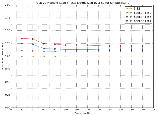
Figure 27: Normalized Flexural Load Effects for Simple Spans
(2-S1-2, Scenario 4, 5 and 6)
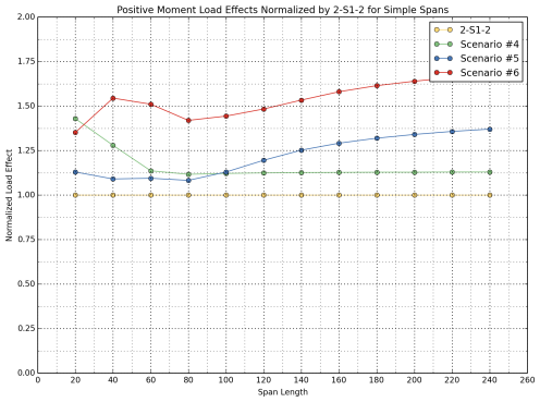
Figure 28: Normalized Shear Load Effects for Simple Spans
(3-S2, Scenario 1, 2 and 3)
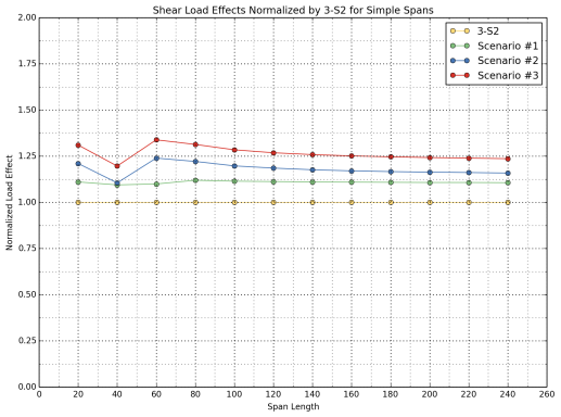
Figure 29: Normalized Shear Load Effects for Simple Spans
(2-S1-2, Scenario 4, 5 and 6)
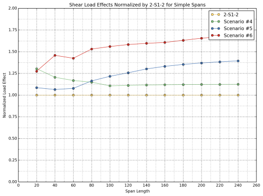
Figure 30: Normalized Flexural Load Effects for Continuous Spans
(3-S2, Scenario 1, 2 and 3)
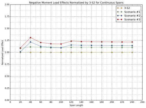
Figure 31: Normalized Flexural Load Effects for Continuous Spans
(2-S1-2, Scenario 4, 5 and 6)
2.6 Summary Findings: Load Effects by Span Length and Scenario
- Scenario 1 consistently yields 10 percent greater load effects (for positive flexure, negative flexure, and shear) than the 3-S2 control vehicle for all span lengths.
- Scenario 2 yields approximately 25 percent greater positive moments when compared with the 3-S2 control vehicle for short spans (less than 60 ft.); however, the difference becomes less pronounced and stabilizes at around 13 percent for spans longer than 60 ft.
For shear load effects, the increase due to Scenario 2 varies between 10 percent and 24 percent for spans shorter than 80 ft. For longer span lengths, the USDOT study team observed a fairly stable trend where the average difference is 17 percent.
For negative flexure, Scenario 2 yields similar load effects at very short span lengths (20 ft. +/-). The difference increases as the span length increases, but stabilizes for spans greater than 40 ft., with an average difference of 14 percent.
- Scenario 3 yields approximately 35 percent greater positive moments than the 3-S2 control vehicle for short spans (less than 60 ft.); however, similar to the behavior observed for Scenario 2, the difference becomes less pronounced and stabilizes at around 20 percent for spans longer than 60 ft.
For shear load effects, the difference varies between 20 percent and 34 percent for spans shorter than 80 ft. For longer span lengths, a fairly stable trend was observed where the average increase is 25 percent.
For negative flexure, Scenario 3 yields 10 percent greater load effects when compared with the 3-S2 control vehicle for very short span lengths (20 ft. +/-). The difference increases with increasing span lengths, but stabilizes to some degree for spans greater than 40 ft., with an average difference of 22 percent.
- Scenario 4 generates around 40 percent greater positive moments than the 2-S1-2 control vehicle for very short spans (20 ft. +/-). The difference diminishes linearly with increasing span lengths, and stabilizes at around 13 percent for spans in excess of 60 ft.
Shear load effects are 30 percent greater than the control vehicle for very short spans (20 ft. +/-); however, the difference is less pronounced as the span length increases, and is stabilized at around 11 percent for spans in excess of 100 ft.
For negative flexure, a similar behavior was observed as with the case for shear. Negative moments are 21 percent higher than the control vehicle for very short spans (20 ft. +/-); however, the difference diminishes with increasing span lengths and stabilizes at around 13 percent for spans in excess of 100 ft.
- Scenario 5 consistently yields 10 percent greater positive moments than the 2-S1-2 control vehicle for spans up to 80 ft. For longer spans the difference in positive moments appears to increase with increasing span length.
For this Scenario shear load effects are about 8 percent greater than for the control vehicle for spans up to 60 ft. For longer span lengths the difference tends to increase as the span length increases.
Negative flexure exhibits a rather complex behavior for the Scenario 5 vehicle. For instance, a maximum increase of 50 percent in the calculated negative moment was observed for a span length of 80 ft.
- Scenario 6 displays a complex behavior for spans less than 80 ft., where the difference between this configuration and the 2-S1-2 control vehicle varies between 35 percent and 55 percent. However, for spans greater than 80 ft., the difference increases as the span length increases, as was the case for Scenario 5.
Shear load effects are around 25 percent greater than the baseline vehicle for very short spans (20 ft. +/-), and tend to increase as the span length increases.
Negative flexure exhibits complex behavior in the case of Scenario 5 where a maximum relative increase of 86 percent in the calculated negative moment over that of the control vehicle was observed for a span length of 80 ft.