3.4 Review of NCHRP 342
To date, the most complete theoretical and mathematical treatment of benefits estimation is in the supplement to NCHRP 342 [3], and particularly in Appendix D. Much of this material is highly technical and not easily accessible to a reader without a strong knowledge of micro-economic theory and a good grasp of mathematics.
3.4.1 Approach and Assumptions
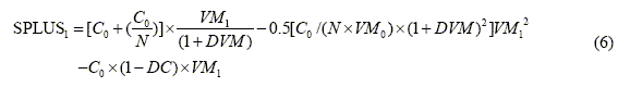
Appendix D to NCHRP Report 342 developed a method to calculate the increase in consumer surplus resulting from a road network improvement. It assumed that road network improvements impact private sector productivity. Transport intensive firms were expected to alter their logistics to take advantage of road network improvements.
The basis for the approach was the assumption that a network improvement results in a shift in the demand curve for transportation. The conventional approach to measuring benefits of infrastructure investment is to estimate the direct cost savings to current users, and add an additional allowance for the benefits of increased infrastructure use caused by the lowered costs. Before the road improvement, current use is![]() VM0 and the cost of operations to users is an average
VM0 and the cost of operations to users is an average![]() C0. Demand for road use is a function of the cost of road use, expressed in $ per vehicle mile. This corresponds to a generalized cost since it includes time, fuel, wear, etc., as well as delays due to congestion. The lower the cost of using the road network, the more it will be used.
C0. Demand for road use is a function of the cost of road use, expressed in $ per vehicle mile. This corresponds to a generalized cost since it includes time, fuel, wear, etc., as well as delays due to congestion. The lower the cost of using the road network, the more it will be used.
After road network improvement reducing congestion, saving time, fuel, and depreciation, the reduced cost per vehicle mile is estimated at![]() C1. Because of the lower cost of using the road, use expands to
C1. Because of the lower cost of using the road, use expands to![]() VM1. For simplicity, the model assumed a linear demand curve, and used the elasticity of demand as its primary input. With P as transport cost C, Q as transport demand VM, and N as the price elasticity of demand, it is possible to write:
VM1. For simplicity, the model assumed a linear demand curve, and used the elasticity of demand as its primary input. With P as transport cost C, Q as transport demand VM, and N as the price elasticity of demand, it is possible to write:
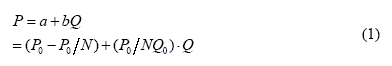
The higher demand curve![]() D′ represents the shift in demand due to logistics re-organization. The combined lower operating costs per vehicle mile and the logistics savings results in volume of use
D′ represents the shift in demand due to logistics re-organization. The combined lower operating costs per vehicle mile and the logistics savings results in volume of use![]() VM2. The benefits are given by the increase in surplus, areas
VM2. The benefits are given by the increase in surplus, areas![]() a+b+c). Under this model, area c is the impact of logistics changes, and would have been missed by previous practice.
a+b+c). Under this model, area c is the impact of logistics changes, and would have been missed by previous practice.
Exhibit 18: Productivity gains due to road improvements.
After re-organization, the new demand curve (shifted), was estimated as:
where a and b are changed to reflect operating costs and demand for transport:
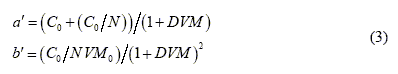
The term DVM was defined as the percent change in road use required by road using firms to provide their clients with the same level of service as before the infrastructure investment. It will be shown later that network improvements result in a progressive extension or tilt of the demand curve vice a shift.
In NCHRP 342, it was also assumed that there were no economies of scale for shippers. That is the per-unit cost of transport did not vary with volume of traffic (transport service used). This was seen as a conservative estimate since cost will tend to fall when serving greater volumes within a given delivery area. This again must be estimated at the level of the firm. The report stated it was possible to improve the algorithm but did not propose a procedure.
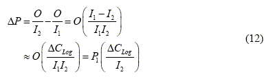
While reviewing Report 342, a problem was identified with the definition and derivation of DC, as the proportional change in operating costs per vehicle mile of use at current volumes or level of service. The problem, stemming from non-additive proportional changes, has been resolved and can be found at Appendix 2. The new expression states that the proportionate change in average cost per vehicle mile is a combination of proportionate savings in transportation and a scaled change in other costs. With this correction, the expression for DC can then be carried forward in the determination of consumer surplus.
3.4.2 Benefits Derivation
The end result of NCHRP 342 was the determination of gains in consumer surplus (areas![]() a+b+c). For the case of a linear demand curve, this was derived as:
a+b+c). For the case of a linear demand curve, this was derived as:
where the surplus before highway improvements is:
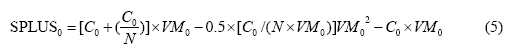
and the after investment surplus is:
The net benefits from an increase in consumer surplus is therefore a function of:
![]() C0 = Initial cost of transport
C0 = Initial cost of transport
N = elasticity of demand
VM = vehicle miles used
DVM = proportional change in vehicle miles
DC = proportional change in logistics costs
An alternate derivation was also provided based on the observation that the new cost of transporting S units can be expressed as:
which says the new cost is proportional to the increase in transportation use as well as the decrease in cost. Assuming suitable estimates can be obtained for all these quantities, it is a simple matter to calculate benefits.
3.4.3 Conclusion
The above derivation suffers from a number of shortfalls. The level of output of the firm remains fixed, an assumption that we wish to relax in a revised framework. A linear demand curve was also assumed, but for small changes in logistics costs, this may be a reasonable approximation. The theoretical framework should hold for any demand curve. Furthermore, it was also assumed that absolute logistics cost savings were known. Some form of aggregation through the estimation of elasticities is required – this was addressed in the follow-on work documented in NCHRP 2-17(4).
The above derivation establishes benefits measurement through a relationship between transportation cost and transportation service (VM), while quantity shipped remained fixed. In fact quantity shipped would be expected to increase thereby improving firm productivity and so a simpler more direct and transparent method to measure benefits is needed.
3.5 Review of NCHRP 2-17(4)
3.5.1 Approach and Assumptions
The methodology in 2-17(4) focused on trade-offs between freight transport and other logistics inputs. Again, constant output of the firm is assumed. Logistics cost savings may allow firms to reduce their price, thereby increasing product demand, sales and transportation used. These relationships are illustrated in the influence diagram at Exhibit 22. The effect of additional demand will be covered in section 4.1.
The shipment is considered the basic unit of transportation provided. It is assumed that there are M types of transportation services available to the firm. The relevant characteristics of a shipment![]() Si = S(Li,Wi,Mi,Vi,TiσTi) are:
Si = S(Li,Wi,Mi,Vi,TiσTi) are:
![]() Li = origin-destination pair (transportation link)
Li = origin-destination pair (transportation link)
![]() Wi = shipment weight
Wi = shipment weight
![]() Mi = transport mode
Mi = transport mode
![]() Vi = Value-added services
Vi = Value-added services
![]() Ti = expected travel time
Ti = expected travel time
![]() σTi = variance of travel time
σTi = variance of travel time
The relationship between logistics inputs and level of service needed to support the production and distribution function of the firm are described by the production function:
where Y is the output of the firm (final sales),![]() Si are the shipments,
Si are the shipments,![]() Ij are the inventory stocks,
Ij are the inventory stocks,![]() Bk are the warehouse spaces, and
Bk are the warehouse spaces, and![]() ITl is an information input related to order processing[14]. As a result of infrastructure investment, characteristics of shipments may change and the firm will seek to minimize its total costs subject to maintaining or improving production.
ITl is an information input related to order processing[14]. As a result of infrastructure investment, characteristics of shipments may change and the firm will seek to minimize its total costs subject to maintaining or improving production.
3.5.2 Benefits Derivation
The measurement of benefits was achieved through a derivation of the total willingness to pay (WTP), in dollars. This WTP is based on aggregate logistics cost savings for like firms and industries.
WTP has been expressed as:
where,
TS = Total sales ($)
![]() αLog = logistics cost as percent of total sales (%)
αLog = logistics cost as percent of total sales (%)
T = average travel time (hours)
![]() σT = variance of travel time (hours**2)
σT = variance of travel time (hours**2)
![]() ηT = elasticity of logistics cost with respect to travel time
ηT = elasticity of logistics cost with respect to travel time
![]() ησT = elasticity of logistics cost with respect to travel time variance.
ησT = elasticity of logistics cost with respect to travel time variance.
The specific form of the dimensionless function F depends on the nature of joint effects of travel time and variability on logistics costs. In the case where savings due to travel time and variability are assumed additive, the expression was written as follows:
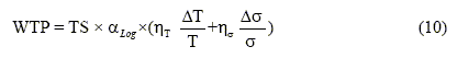
An alternate derivation of WTP was proposed for the case where a complementary relationship exists between travel time and reliability. Since it was not used, we do not discuss it further here. The above derivation for WTP was used to calculate changes in the firm's logistics costs via sampled elasticities. This function could be generalized to also include other effects of highway improvements such as heavier loads, larger capacity trucks, and changes in hours of service.
Sampled Elasticities
It is not practical to attempt to quantify each firms "absolute" logistics cost savings. What is possible, rather, is to qualify the nature and extent of logistics re-organization for a statistical sample of firms and to infer elasticities as a measure of their response to infrastructure improvements. The error in the slope of the curve (elasticity) can be estimated and controlled based on the variability of the sample. A cost-effective solution can then be found for the estimation process itself.
There is a requirement for systematic and transparent interviews of firms' logistics planners to obtain information on the impact of transportation cost reductions. The points at which re-organization occurs and its extent is also required as part of the sample. As is demonstrated at Exhibit 19, re-organization creates a jump gain in proportional logistics cost savings at specific levels of time savings. There could be several steps at which savings occur – one for inventory policy changes[15], a second for warehouse consolidation as part of logistics system changes.
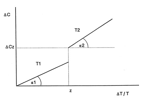
Exhibit 19: Cost Savings by firm for relative changes in travel time.
The aggregate savings can be computed for the sample of firms, as shown at Exhibit 20. The aggregate cost savings function was shown to be
![]()
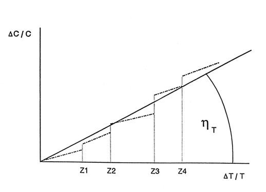
Exhibit 20: Aggregate industry relative cost savings and estimation of elasticity.
Given total sales, logistics costs as a proportion of total sales, elasticity of logistics costs with respect to travel time and travel time variability, the willingness to pay, WTP, can be computed by commodity across various industries.
3.5.3 Productivity Gains
Although the BCA framework will capture productivity effects, we expand on the description provided in NCHRP 2-17(4) to relate productivity gains to logistics cost savings.
Once firms identify ways to reduce costs and restructure their logistics as a result of better highways, they will combine inputs in a different way to produce the same level (or more) of output. Restructuring can be seen as a more efficient employment of resources. In this case, it is possible to quantify changes in firms' productivity.
Productivity is the ratio of outputs to inputs. This can be written
A change in productivity may occur as a result of logistics restructuring. This change is given by:
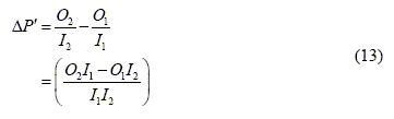
Productivity gains can then be expressed in terms of previous productivity and relative logistics savings with respect to the new input level. For the case of changing output, productivity gains![]() ∆P′ can be written as:
∆P′ can be written as:
Productivity gains can be realized as a result of improved transportation infrastructure. Benefits from these gains will be captured as part of net benefits in the BCA framework to be developed later in the report. Even if productivity gains are a useful indicator of the value of infrastructure investment, they are not an addition to what is reported in net benefits in the proposed approach.
3.6 Critique of Developments to Date
The scope and general approach of previous HLB studies can be seen from the revised influence diagram at Exhibit 22 below. The focus and scope of each study is highlighted with an area covering the primary variables and their relationships in deriving total benefits. NCHRP 342 considered logistics cost savings, and the shift in demand for transport, while NCHRP 2-17(4) considered net logistics cost savings as a function of travel time and travel time variability changes.
With this work, we are attempting to build on previous studies while letting the firm's output vary. In measuring infrastructure improvement benefits, improved firm productivity will be an important effect to capture. Industrial re-organization can lead to reduced logistics costs that can be passed on to consumers thereby increasing product demand.
In the first instance, NCHRP 342 assumed a shifting demand curve for transportation services. This implies that if, for whatever reason, the price increases back to its old level, demand would be higher than originally. One could imagine such a case but only in the very short run. In the long run, the process should be reversible.
What is more plausible is an outward sloping demand curve given the opportunity for firms to re-organize their logistics over time. Exhibit 21 indicates the demand D for transportation given no re-organization effect. With re-organization, the demand for transportation, noted![]() D′, may increase at any given price level. "By how much" is an essential question which will help solve the overall benefits assessment problem. In the Exhibit below, area a represents the immediate direct benefit to a firm. It is the cost savings based on current road use, while area b is the medium run net value of the increase in road use (possibly due to changes in inventory). Area c represents the benefit from a longer run response to logistics re-organization such as for warehouse consolidation or other long-term changes.
D′, may increase at any given price level. "By how much" is an essential question which will help solve the overall benefits assessment problem. In the Exhibit below, area a represents the immediate direct benefit to a firm. It is the cost savings based on current road use, while area b is the medium run net value of the increase in road use (possibly due to changes in inventory). Area c represents the benefit from a longer run response to logistics re-organization such as for warehouse consolidation or other long-term changes.
The second major study, NCHRP 2-17(4) addressed net benefits as a willingness to pay for overall logistics cost savings. With this approach, it is difficult to address possible increases in product demand and the effects of marginal cost pricing. A more conventional approach based on consumers surplus is seen as better suited. As we shall see in the proposed framework, however, elements of 2-17(4) will be retained in the determination of firms' responses to infrastructure investments and elasticity estimation.
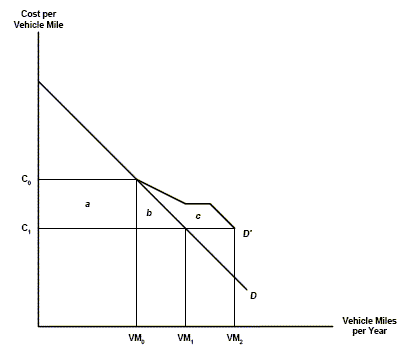
Exhibit 21: Demand curve as affected by logistics re-organization.
3.7 Conclusion
The overall framework described in the next section shall be based on a variant of the shifting demand curve method from NCHRP 342 for the change in consumer surplus, as well as elements of NCHRP 2-17(4) for elasticity estimation. This is to be enhanced with strategies to allow for changes in output of final products, absence of marginal cost pricing, and presence of possible monopolies.
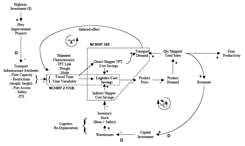
Exhibit 22: Freight economics influence diagram and previous studies.