Work Zone Mobility and Safety Program

Work Zone Application of Bluetooth Traffic Detection

slide 1: Work Zone Application of Bluetooth Traffic Detection


FHWA Work Zone Peer Exchange, Atlanta, GA

May 8, 2013

John W. Shaw, P.E.
Traffic & Data Microsimulation Manager
Wisconsin Traffic Operatiosn and Safety Laboratory


slide 2: Would You Like To...


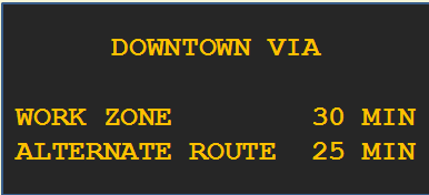
  • Know when traffic in your work zone is starting to slow down?
  • Provide travel times for alternate routes?

This image shows a dyanmic message sign providing travel times to downtown for the work zone and alternate routes.


slide 3: Would You Like To…


  • Compare actual work zone delay with what was predicted in the TMP/MOT?
  • Evaluate locational differences in work zone throughput?
  • See how much traffic diverted to the alternate route?
  • See whether people who diverted actually saved time?


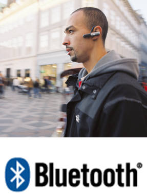
slide 4: What is Bluetooth?


  • 2.4 GHz wireless system for connecting electronic devices.
  • Low power, low cost.
  • Range ∼100 meters.
  • High level of data/content security.
  • Every device has unique MAC address.
  • No master database of MAC addresses.
  • Used for traffic detection since 2008.

A man wearing a Bluetooth headset above the Bluetooth logo.


slide 5: Bluetooth Data Collection


The Bluetooth data collection framework.  A field device with a Bluetooth receiver and cellular modem detects the Bluetooth-enabled handsfree kit in a passing car.  The field device relays this information to the database server for reporting and analysis.


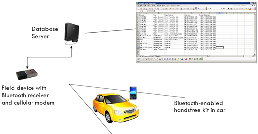
slide 6: Bluetooth Data Collection


A central server notes the time and location stamps when a vehicle passes Detectors A and B.  The detector uses the time and location stamps to calculate the vehicle's average speed between the detectors.  The detectors identify the vehicle by the unique MAC ID of the vehicle's Bluetooth equipment.


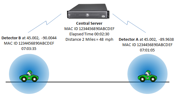
slide 7: Vehicle Re-Identification Process


  1. "Listen" for Bluetooth MAC addresses at two or more locations.
  2. Record observation time and location.
  3. Transmit observations to central server.
  4. Match MAC addresses spatially.
  5. Compute travel time.
  6. Filter out unreasonable travel times.
  7. Evaluate and Report Speed, OD and Route.
  8. Combine with volume data if appropriate.


slide 8: What Can Bluetooth Do?


  • One Detector:
    • Not Much
  • Two Detectors:
    • Trip Time (Speed)
  • Three Detectors:
    • Origin and Destination
  • Four or More Detectors:
    • Route Choice
The increasing capabilities as the number bluetooth detectors inceases.  One detector cannot do much.  Two detectors can be used to calculate trip time or speed.  Three detectors can be used to identify trip origin and destination.  Four or more detectors can be used to identify route choices.


slide 9: By Itself, Bluetooth Provides…


  • Discrete, time-stamped observations of people/vehicles moving around.
  • But NOT traffic volume.

A road tube traffic counter.


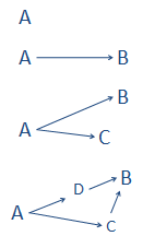
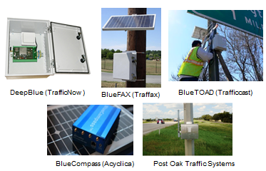
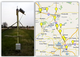
slide 10: Field Equipment


The inside of a field detector unit.


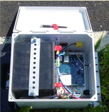
slide 11: Installation


Two workers installing a detector onto a roadside sign.


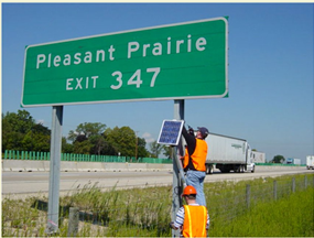
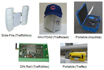
slide 12: Equipment Set-up


A workers setting up a detector that has been mounted on a roadside structure.


slide 13: Cabinet-Mount Examples


Collage of photos including the DeepBlue cabinet-mount manufactured by TrafficNow, the BlueFAX cabinet-mount manufactured by Traffax, the BlueTOAD cabinet-mount manufactured by Trafficcast, the BlueCompass cabinet-mount manufactured by Acyclica, and the Post Oak Traffic Systems cabinet-mount.


slide 14: Other Configurations


Collage of photos including the Side-Fire detector manufactured by TrafficNow, the MiniTOAD detector manufactured by Trafficcast, a portable detector manufactured by Acyclica, the DIN Rail detector manufactured by TrafficNow, and a portable detector manufactured by Traffax.


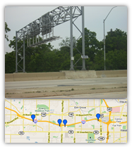
slide 15: Travel Time – Western Milwaukee Suburbs
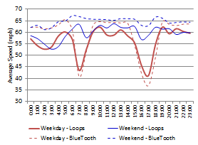

  • 5.5 mile segment carrying 130,000 AADT
  • WisDOT concerned about accuracy of DMS travel times
  • Current system using data from 41 loop detectors
  • Some loops reporting zero speeds
  • Speeds sensitive to ongoing calibration
A photo of a detector mounted to an overhead guide sign structure is placed above a map showing four detector locations on the Interstate 94 corridor west of Milwaukee, Wisconsin.


slide 16: Findings


  • Loop speeds low in free-flow conditions
  • Loop speeds too high in congestion
  • BT pairing sampling rate <3% (2010)

Chart plots vehicles' average speeds on the vertical axis and the time of day on the horizontal axis. The chart plots 4 data sets: weekday drivers logged by loop detectors, week day drivers logged by BlueTooth detctors, weekend drivers logged by loop detectors, and weekend drivers logged by BlueTooth detectors.  Weekday drivers' average speeds slowed to about 45 miles per hour during morning rush-hour (7:00 AM) and about 40 miles per hour during evening rush-hour (5:00PM).


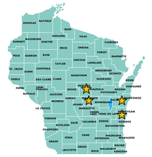
slide 17: Recent Work Zone Field Studies


  • Milwaukee
  • Portage
  • Grafton
  • Endeavor

A map  highlighting the location of 4 recent work zone field studies: Milwaukee, Portage, Grafton, and Endeavor.


slide 18: Work Zone Traffic Performance


A three-step flow chart for work zone traffic performance. The chart begins with demand, which leads to capacity, which leads to diversion.


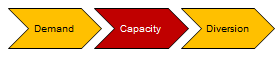
slide 19: Freeway Work Zone Capacity


Why do some work zones operate better than others?

Two side-by-side images, one of a traffic camera image of work zone-related congestion, the other a chart showing travellers' average speed on the vertical axis and the flow rate (number of vehicles per hour per lane) on the horizontal axis.  The chart plots the speed and flow rate for an interstate corridor and a congested corridor.  It also plots the work-zone speed-flow curve through both data sets.


slide 20: Rural Freeway WZ Capacity, Delay & Route Choice (Portage, WI)


  • Weekend recreational route
  • 30+ miles
  • 13 BT units
  • Mainline + Alternates
  • Volume counts

Two side-by-side images, one of a photo of a roadside detector and the other of a map of the I-90/I-94 corridor in Wisconsin, between Madison and Portage.  The map shows locations of BlueTooth detector units.


slide 21: Results: Rural Freeway Capacity


Chart plots two data sets based on the time of day (the horizontal axis). The first data set shows freeway volume which peaks during increases during business hours, peaking from 12:00 PM until about 10:00 PM, then declining. The second data set shows freeway speed in miles per hour.  Stable flow of 65 to 70 miles per hour) obtains until 12:00 PM (when traffic volume peaks).  As traffic volume peaks at approximately 1625 vehicles per lane per hour, freeway speed decreases from 70 miles per hour at 12:00 PM to approximately 25 miles per hour from approximately 4:00 PM to 7:00 PM.  Queue discharge begins at approximately 5:00 PM and freeway speed begins to recover approxmiately 7:00 PM to 9:00 PM.


slide 22: Results: Rural Route Choice


  • Drivers can respond to WZ congestion in a variety of ways.
  • Modest increases in traffic on alternate routes
  • Relatively few exited and then returned to freeway.
  • More commonly, local traffic stayed on local routes until past the work zone.

A map of the I-90/I-94 corridor in Wisconsin, between Madison and Portage.  The map shows locations of BlueTooth detector units.


slide 23: Urban Freeway WZ Capacity, Delay & Route Choice (Milwaukee Suburbs)


  • Freeway Mainline + Two Alternate Routes
  • Bluetooth Detectors + Volume Counts

A map of the I-94 corridor, west of Milwaukee, Wisconsin.  The map highlights I-94 going west from western suburbs of Milwaukee.


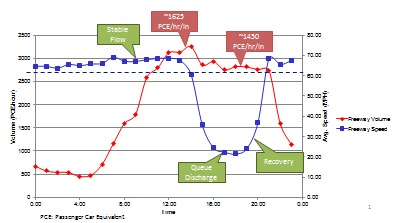
slide 24: Results: Urban Freeway Capacity


Chart plots two data sets based on the time of day (the horizontal axis). The first data set is traffic volume which peaks, then decereases during the morning (6:00 AM to 9:00 AM) and afternoon (3:00 PM to 6:00 PM) rush hour periods.  Average speeds remain steady between 55 and 60 miles per hour until approximately 6:00 AM, drop to approximately 20 miles per hours during the morning rush hour, recover mid-day, then drop to approximately 30 miles per hour during the evening rush hour.

Stable Flow

AM: 1825-2200 PCE/hr/lane
PM: 1825-1950 PCE/hr/lane

Queue Discharge

AM: 1600-1825 PCE/hr/lane
PM: 1725-1825 PCE/hr/lane


slide 25: Results: Urban Route Choice


A map of the I-94 corridor, west of Milwaukee, Wisconsin.  The map highlights I-94 going west from western suburbs of Milwaukee.

  • Commuters very willing to use alt routes.
  • Increased traffic on alt routes even when mainline was not congested.


slide 26: Lessons Learned


An overhead image of 5-lane restricted access highway with a circular highlighted area focused on the right-hand lane.

slide notes:

None.


slide 27: Lessons Learned


An overhead image of 5-lane restricted access highway with an elliptical highlighted area focused on the right-hand lane.


slide 28: Lessons Learned


  • Detection rates vary by route type and time of day.
  • Since Jan 2012, USDOT requires truck drivers to use hands-free devices.


slide 29: Data Processing Matters


A scatter-plot of the trip times on the vertical axis and the date and time of travel on the horizontal axis.  The data shows bluetooth observations of travel times from South Lake Tahoe, California to Placerville, California.  The most dense distribution of travel times frall from appriximately 50 to 100 minutes with decreasing densities for longer travel times.
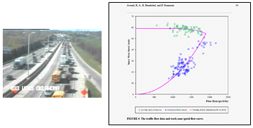
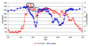
Figure 13. Raw Observations, US-50, South Lake Tahoe, CA to Placerville, CA


slide 30: The Secret is in the Software


Options

  • Proprietary vendor-supplied filtering and matching services
  • Free software from sensor vendors (basic)
  • Third-party software (advanced)


slide 31: Bluetooth vs. Side-Fire Radar


Bluetooth

  • Speed (lagging)
  • Travel time for a route segment
  • Accurate at all speeds
  • Many mounting options
  • Observes all traffic
  • Low power consumption
  • Requires at least 2 detectors
  • $2500-5000 per detector
  • Some vendors offer rental

Radar

  • Speed + Volume
  • Point speed at a specific location
  • Not accurate at low speed
  • Pole-mount at roadside
  • Observes specific lanes
  • 8 to 11 watts continuous
  • Can get data from a single detector
  • About $5000 per detector


slide 32: Bluetooth Pro & Con


Strengths

  • Inexpensive
  • Low power consumption
  • Highly accurate speed data
  • Easy to extend study duration
  • Efficient method for collecting OD info
  • Only practical way to collect route choice data

Limitations

  • Low sampling rates
  • Capture rates can vary by time of day (prob. trucks)
  • Sometimes sensitive to:
    • Site Characteristics
    • Antenna Placement
    • Loss of Power/Comm
    • Data processing assumptions


slide 33: Questions?


slide 34: Presenter Contact Information


John W. Shaw

jwshaw@wisc.edu
414-227-2150


Return to List of Presentations
Office of Operations