Appendix E: Vehicle Entry Headway Generation in CORSIM
When injecting vehicles into a network at an entry node, CORSIM can generate vehicle entry headways deterministically or stochastically, using one of several distribution types. In the deterministic mode, vehicles are injected into the network at with a constant headway. In the stochastic generation mode, CORSIM uses a random sampling of a user-selected distribution to generate vehicle entry headways.
Deterministic Mode
In the deterministic mode, vehicles are injected into the network at with a constant headway, defined as 3,600 divided by N, where N is the hourly volume in vehicles/hour defined for the entry node. As expected, using a constant headway generates a constant flow of vehicles into the network with a constant temporal spacing between entering vehicles.
Stochastic Mode
In a real traffic network, vehicles do not generally travel with a constant headway. Therefore, it is more realistic to inject vehicles into a simulated network by using non-constant headways. By using a random distribution of headways, the analyst can replicate platoons of vehicles when injecting vehicles into the network. Such groupings of vehicles are often seen in the real world.
In the stochastic mode, CORSIM uses a random sampling of a user-selected distribution to generate vehicle entry headways. This process does not vary the number of vehicles emitted each run; only the headways between the vehicles are varied. The constant headway, defined in the previous paragraph, serves as the mean value for a user-selected distribution function. The analyst can select from one of three types of distributions: normal (Gaussian), negative exponential, or Erlang.
Normal Distribution
The normal (Gaussian) distribution is often selected for a stochastic process as an approximation of more complex distributions, or when little else is known about the true distribution of a random variable beyond its mean and variance.
When the analyst selects the normal distribution for generating vehicle entry headways, the mean value for the distribution is defined as 3,600 divided by N, where N is the hourly volume in vehicles/hour defined for an entry node. CORSIM defines the standard deviation for the distribution as the difference of the mean and minimum headway values divided by 2.575. This definition is a holdover from the old lookup table logic and effectively defines the minimum value to be 2.575 standard deviations from the mean.
Figure 71 illustrates a normal distribution, generated by CORSIM using a volume of 480 veh/h. The mean and standard deviation for the distribution are calculated as described in the preceding paragraph. A minimum value of 1.2 seconds is used.
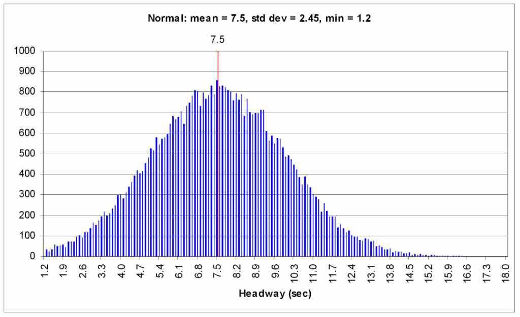
Figure 71 . Graph. Normal distribution.
Negative Exponential Distribution
The negative exponential distribution is a specialization of the gamma (and Erlang) distribution, and is commonly used for generating the inter-arrival time of “customers” to a system. Figure 72 illustrates the histogram for the negative exponential distribution, generated using the inverse-transform method. The mean headway is 7.5 seconds and minimum headway is 1.2 seconds in this example.
In the absence of field measured headways, analysts should use a negative exponential distribution for real-world applications.
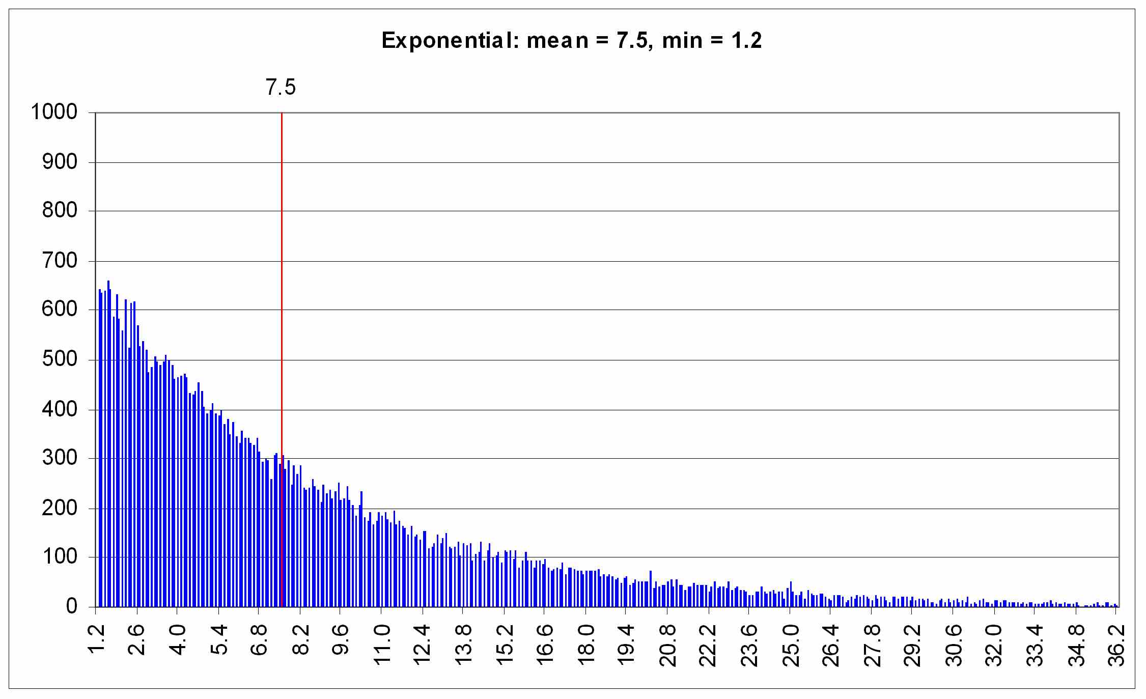
Figure 72 . Graph. Exponential variates.
When the analyst selects the negative exponential distribution for generating vehicle entry headways, the mean value for the distribution is defined as 3,600 divided by N, where N is the hourly volume in vehicles/hour defined for an entry node.
Erlang Distribution
The Erlang (sometimes called m-Erlang) distribution is a specialization of the gamma distribution, and is commonly used for generating the time required to complete some task.
When the analyst selects the Erlang distribution for generating vehicle entry headways, the mean value for the distribution is defined as 3,600 divided by N, where N is the hourly volume in vehicles/hour defined for an entry node. Furthermore, the analyst can specify the value of the Erlang distribution shape parameter to be used in generating vehicle entry headways. Figure 73 illustrates the Erlang distribution for several values of the shape parameter, a, and for a mean value of 1.
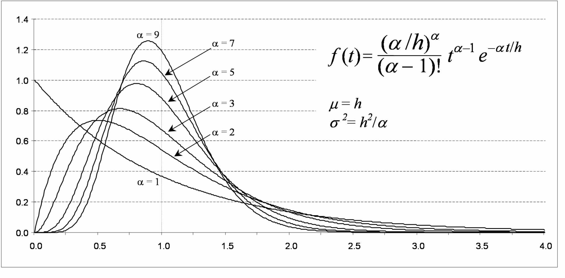
Figure 73 . Graph. Erlang distribution.
The equation for the Erlang headway distribution is included in the Erlang distribution figure, where t represents the headway and h is the mean (average) headway computed as previously described. The shape parameter, a, describes the level of randomness of the distribution ranging from a = 1 (most randomness) to a = ¥ (constant value at the mean). When a = 1, the Erlang distribution is equivalent to the negative exponential distribution. CORSIM can generate headways from Erlang distributions ranging from a = 1 to a = 9.
The entry headway is a global parameter in CORSIM, meaning the parameter cannot be set differently for individual links or subnetworks, and the default setting is a constant headway. However, a stochastic distribution (Normal or Erlang) would be more appropriate for real-world applications to account for natural randomness in vehicle headways. In the absence of field measured headways, an Erlang Distribution with a = 1 may be used, which equates to a negative exponential distribution. A negative exponential distribution is commonly used for generating the inter-arrival time of “customers” (e.g., vehicles) to a system.