Weather Applications and Products Enabled Through Vehicle Infrastructure Integration (VII)

7. Potential VII Products and Applications

WEATHER AND ROAD CONDITION IMPROVEMENTS ENABLED BY VII

In this section, weather and road condition product concepts enabled by vehicle data and/or improvements in weather and road condition products due to the utilization of vehicle data are presented. The examples presented herein were selected because it was felt that they were particularly relevant to the surface transportation community. Surface transportation stakeholder categories that will benefit from weather and road condition products enhanced with vehicle data include, but are not limited to:

• Traffic management
• Incident management
• Maintenance (winter and non-winter)
• Travelers
• Emergency management

The general assumption for this section is that the vehicle data are valid, that is, they have sufficient quality to be utilized in the product concepts described herein. Ideas about the type of methods and techniques that may be required to develop these product concepts are discussed in Section 9.

7.1 Weather Product Improvements Enabled by VII

Several examples of weather products that will be improved with vehicle data are presented in this section. The examples are not exhaustive and only provide a sampling of what will be possible with these new datasets. The product examples include both improvements in the diagnoses of current weather conditions and in weather prediction. The primary potential contribution of vehicle data will be its ability to help characterize the lowest levels of the atmospheric boundary layer as well as pavement conditions.

Weather improvements that will be enabled with vehicle data include, but are not limited to:

• Reducing radar anomalous propagation (AP)
• Improved identification of virga (precipitation not reaching the ground)
• Improved identification of precipitation type
• Improved identification of foggy regions
• Improved characterization of surface conditions for weather models
• Improved weather analysis and prediction in complex terrain
• Improved air quality monitoring and prediction
• Improved diagnosis of boundary layer water vapor
  

7.1.1 Reducing Radar Anomalous Propagation (AP)

Doppler weather radar data are used widely for many weather applications and products throughout the country. The NWS and DOD operate 158 NEXRAD Doppler weather radars throughout the country. Several sophisticated radar data quality algorithms have been implemented to reduce artifacts such as ground clutter, point targets, and anomalous propagation, but there are still times when data quality suffers from contamination (18, 19).

FIGURE 7.1. Doppler weather radar mosaic showing intensity (reflectivity) at Aberdeen, South Dakota on 15 March 2002 at 02:19 UTC. The image illustrates the impact of anomalous propagation (AP) on data quality.⁸ Although echoes are displayed in the image, no precipitation was occurring at the ground. None of the echoes displayed are precipitation.

Figure 7.1 is a radar intensity image from Aberdeen, South Dakota from 15 March 2002. Although the image suggests that light precipitation is falling in central South Dakota, no precipitation was reported. The false return was primarily caused by anomalous propagation (AP), whereby the radar beam was bent toward the ground due to a temperature inversion or water vapor discontinuity in the lower atmosphere. Without widespread surface observations, it is often difficult to confirm whether the radar return is real or an artifact. All users of weather radar data are affected in these situations, as it is difficult to determine if the precipitation is real. DOT winter maintenance personnel, who routinely use radar data to guide tactical decision-making, take appropriately conservative measures to begin winter maintenance operations when precipitation is anticipated. If the radar information turns out to be an artifact, the resources used to begin snow and ice control operations are wasted. Anomalous propagation is not rare and often occurs after precipitation, on clear nights, and after the passage of shallow cold fronts when temperature inversions and/or atmospheric water vapor discontinuities are present.

One of the easiest ways to determine if AP is occurring is to analyze other weather observations to see if there is any corroborating evidence for precipitation. Surface observations and satellite imagery are often used by trained meteorologists and sophisticated algorithms to identify, suppress and/or remove AP from radar data. One limitation of the surface observation network is the low density of observations, particularly when compared to the spatial resolution of radar data samples, which is approximately 1 km (0.62 miles).

VII Contribution: Data from vehicles would help determine if precipitation is occurring in the area in question. The density of vehicle observations will surpass the density of traditional surface observations by several orders of magnitude providing a data rich environment. A direct measurement of precipitation (yes/no) from a vehicle based precipitation sensor would be the best data element to use for this application, but an indirect indication of precipitation from windshield wiper settings could also be used to diagnose the presence of precipitation. Temperature data from vehicles could be used as supplementary input to AP suppression algorithms that are currently applied to radar data by commercial weather vendors.

Challenges: The primary challenge associated with using vehicle data for this application is the uncertainty of how wiper systems are used as was noted in section 5.4. Statistical processing can be used to remove outliers such as when people are using wipers to clean the windshield. The more challenging problem is the use of wipers by a large population of vehicles to address splash-back from wet roads when there is no precipitation. This scenario could lead to AP not being suppressed when it should be because the algorithm may indicate that precipitation is occurring or is likely to be occurring. The majority of time, however, AP will occur in clear conditions, and in these circumstances the use of vehicle data will be more straightforward and have a positive impact.

Vehicle Data Applied to Reducing Radar Anomalous Propagation

Relevant Data Elements	Processing Summary	Primary Challenges
Time	Precipitation sensor and/or wiper setting could be used along with other meteorological datasets to diagnose the presence of precipitation. The vehicle data will be one of many inputs to AP suppressing algorithms.	Identifying occasions when wipers are used or precipitation sensors are responding to splash-back when no precipitation is occurring. If a rain sensor is used as the primary data source, one has to be aware that it will not likely record frozen precipitation.
GPS Location
Precipitation Sensor
Windshield Wipers (front) On/Off
Outside Air Temperature

7.1.2 Improved Identification of Virga

Doppler radars use specific volume scan strategies in an attempt to sense precipitation. The most common strategy, volume coverage pattern 21 (VCP-21), is where the radar makes nine elevation scans from 0.50o to 19.5o every six minutes. As the radar transmits energy at each of these elevations or beam angles, it is also rotating 360 degrees. In some situations, the radar may be accurately sensing precipitation, but the precipitation may not be reaching the ground. Precipitation that does not reach the ground is called virga. When the lower atmosphere is dry, the likelihood of virga increases.

Users of weather radar data are very aware that occasionally the radar data may indicate widespread precipitation when no precipitation is reaching the ground. This situation can last for hours and it is difficult for users to determine if and when the precipitation will reach the ground. This is not a radar artifact as the radar is correctly measuring precipitation. Transportation maintenance (winter and non-winter) and traffic management personnel require accurate radar products to plan operations. Travelers also need accurate surface precipitation information.

VII Contribution: The most direct method of determining whether the precipitation is reaching the ground is to look at surface observations; however, the density of surface observations of precipitation is very low, particularly in remote areas. Vehicle data would be used to supplement standard precipitation observations. Windshield wiper and rain sensor data would be used to determine if precipitation is reaching the ground and that information could be used to adjust and calibrate radar products. This product concept is demonstrated in Figure 7.2 where a radar image from the Front Range NEXRAD (near Denver, Colorado), shows light precipitation northeast of Denver along the I-76 corridor. There are few surface observation stations in the region, so transportation system users would not be able to determine if the measured precipitation was reaching the ground. If vehicle measured wiper setting and/or rain sensor data were available, these data would be used to diagnose the actual presence of precipitation at the ground.

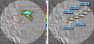
FIGURE 7.2. Denver NEXRAD radar image from 9 February 2006 showing virga in northeast Colorado (left image). Conceptual illustration (right image) of an improved surface precipitation product showing no precipitation at the ground based on an algorithm that correct the product by taking advantage of vehicle data from vehicles traveling along I-76.

Challenges: The primary challenge associated with using vehicle data for this application is the uncertainty of how wiper systems are used. Statistical processing can be used to remove outliers such as people using wipers to clean the windshield. The more challenging problem is the use of wipers by a large population of vehicles to address splash-back from wet roads when there is no precipitation. This scenario could lead to false positive reports of precipitation and the precipitation product not being corrected when it should be.

Vehicle Data Applied to Improving the Identification of Virga

Relevant Data Elements	Processing Summary	Primary Challenges
Time	Precipitation sensor and/or wiper setting would be used along with other meteorological datasets to diagnose the presence of precipitation. The vehicle data will be used to adjust/calibrate the radar data and products.	Identifying occasions when wipers are used or precipitation sensors are responding to splash-back when no precipitation is occurring. If a rain sensor is used as the primary data source one has to be aware that it will not likely record frozen precipitation.
GPS Location
Precipitation Sensor
Windshield Wipers (front) On/Off

7.1.3 Diagnosis of Precipitation Type

Transportation professionals frequently cite precipitation type as one of the most important weather factors influencing the transportation system as it impacts mobility and safety. Identification of the rain/snow boundary is a challenge for the meteorological community as subtle changes in the atmospheric boundary layer such as air temperature, humidity, and precipitation rate can have a dramatic affect on precipitation type.

The Doppler radar technologies utilized throughout the country today (e.g., NEXRAD, media radars, and Terminal Doppler Weather Radars) do not have the ability to directly measure precipitation type. Radar intensity is based primarily on the size of precipitation particles and secondarily on the number of precipitation particles. Advanced weather radars with dual-polarization capability do have the ability to diagnose precipitation type by measuring the shape of the precipitation particles, but it will be many years (approximately 5-10 years) before this new technology is implemented broadly across the nation. In the meantime, precipitation type will continue to be diagnosed using a combination of observational data and weather model analyses.

The lack of a dense surface observation network makes it difficult to generate a high-resolution precipitation type product. Today, precipitation type products often include a broad area designated as mixed precipitation, which generally means that the precipitation may be liquid (rain) or frozen (snow, ice pellets, or freezing rain). The lack of certainty about the precipitation type impacts transportation operations, particularly winter maintenance, as personnel must assume the worst-case scenario and mobilize snow and ice control assets.

The addition of dual-polarization technology on the nation's WSR-88D network and the addition of new low-power local radars with dual-polarization, such as the Collaborative Adaptive Sensing of the Atmosphere (CASA) radar, will significantly improve the ability to diagnose precipitation type. Even with those new technologies in place, precipitation type observations taken from vehicles will be beneficial as these observations will be used as verification data to calibrate the radar algorithms and as input to more sophisticated precipitation type algorithms that combine multiple datasets including radar, surface observation, and model analyses and forecasts.

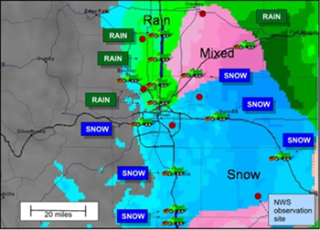
FIGURE 7.3. Illustration of a precipitation type product near Denver, Colorado from October 2005 overlaid with conceptual observations taken by winter maintenance vehicle drivers. The vehicle observations, which would supplement the standard surface observations, could be used by precipitation type diagnosis algorithms to improve the temporal and spatial resolution of the product. The locations of NWS surface observations stations are shown as circles.

VII Contribution: Vehicle data would be used to improve the diagnoses of precipitation type. Surface air temperature is one of the primary factors in the diagnosis of precipitation type, so air temperature data from vehicles would supplement traditional surface observations. The inclusion of vehicle based air temperature observations in precipitation type diagnosis algorithms would improve the spatial and temporal resolution of precipitation type products.

In addition to vehicle measured air temperature observations, direct observations of precipitation type as determined by drivers of winter maintenance vehicles would be beneficial. On-board technologies now exist that allow drivers to input and transmit both sensor-measured and driver-observed weather and road condition information to a central DOT information system. The driver-based observations would be treated as high quality surface observations and be utilized by algorithms designed to diagnose precipitation type over a broad region.

This product concept is illustrated in Figure 7.3 for a winter storm event that occurred in Denver, Colorado in October 2005. The precipitation type product shown in Figure 7.3 is based on a combination of standard NWS surface observations (at airports near Denver), Doppler weather radar, and weather model analyses. The location of NWS surface observation sites is shown as small circles and in this example, six surface observation sites (airports) were utilized in the precipitation type algorithm. The distance between surface observations range from approximately 20 miles to more than 50 miles. Outside of the Denver area, the lack of surface observations significantly affected the quality of the precipitation product since surface observations carry significant weight in the precipitation type algorithm.

If precipitation type information from vehicles were available, the temporal and spatial resolution of the product would be improved as the number and distribution of observations would exceed the fixed observational sites. Anecdotal feedback obtained from transportation authority personnel near Denver for this event suggested that the actual precipitation type did not always match the reported precipitation type particularly for locations away from the NWS reporting sites. This discrepancy is illustrated conceptually in Figure 7.3 where several vehicle-based observations disagree with the analyzed precipitation type.

Challenges: The primary vehicle data elements that would be utilized in this case are air temperature and manual observations of precipitation type. Because precipitation type is highly sensitive to surface air temperature, the quality of the vehicle air temperature would need to be very high. Just a one degree error in a surface air temperature measurement could result in an error in the diagnosed precipitation type. It is very likely that a statistical approach would need to be utilized to ensure that the vehicle based air temperatures represent the predominant condition in the region of interest.

One would expect that human observations of precipitation type from vehicles would be quite accurate; however, this may not always be the case. If this capability were realized, it would be very important that the observations be recorded at the right place and time and not displaced. For example, a driver may observe snow, but not enter the observation into the on-board system until some time later, which could result in the wrong time and location information being tagged to the observation. It is likely that statistical processing would mitigate these issues, but they may still present a concern.

Vehicle Data Applied to Diagnosing Precipitation Type

Relevant Data Elements	Processing Summary	Primary Challenges
Time	The outside air temperature would be used to supplement standard surface air temperature observations from fixed locations (e.g., NWS and RWIS sites) and be utilized in precipitation type diagnosis algorithms. Manual observations of precipitation type taken by transportation operations personnel would be utilized by precipitation type diagnosis algorithms.	Precipitation type is very sensitive to surface air temperature; therefore, the accuracy of the vehicle-based outside air temperature data needs to be high. Data entry errors could impact the resulting precipitation type product.
GPS Location
Outside Air Temperature
Manual observation of precipitation type taken by transportation operations personnel

7.1.4 Identification of Foggy Regions

Fog has been cited as a primary factor in multiple deadly and spectacular crashes (20). It often forms quickly and unexpectedly and often is limited in geographic extent. Fog is difficult to detect and predict because very slight changes in humidity and air temperature (fractions of a degree or percent, respectively) can trigger fog formation. Satellite detection of fog is difficult because cloud layers above the surface can mask lower layers. Infrared satellite processing techniques can be used to identify fog by comparing cloud (fog) top temperatures with ambient air temperature profiles. If the cloud top temperature is at or near the surface air temperature, then the cloud is diagnosed as fog. This approach is satisfactory for many applications, but not necessarily for surface transportation where fog has to be at eye level and very dense before drivers will take notice. Drivers typically do not modify their driving behavior until the visibility is less than a few hundred feet.

The meteorological community has not been able to demonstrate a lot of skill in diagnosing or predicting fog density or visibility. Visibility depends on several factors including cloud droplet size and concentration, water vapor saturation level, aerosol characteristics, and viewing angle relative to the primary light source (e.g., sun). Fog mitigation strategies for surface transportation usually involve the implementation of visibility sensors in areas prone to fog. This works well if the foggy regions are somewhat predictable, such as over waterways, valleys, or near industrial complexes that emit water vapor.

Fog and visibility detection/diagnosis and prediction could be improved with more dense and frequent surface observations of visibility, humidity, and air temperature. Because the formation of fog is highly sensitive to several variables, high quality observations are required.

FIGURE 7.4. Conceptual illustration of vehicle data along a roadway in Kansas whereby the vehicles are moving through a foggy region. In this example, vehicle data contributing to a fog product include speed, relative humidity, headlamp setting, outside air temperature (OAT), and brake usage.

VII Contribution: Vehicle data will provide an opportunity to improve fog diagnosis and prediction, but there are many challenges. Visibility measurements would provide the most direct indication of fog, but visibility is not a current or planned vehicle data element. Relative humidity measurements would also be used to diagnose fog, but are not available on standard vehicles. If a humidity data field (e.g., relative humidity, absolute humidity, water vapor mixing ratio, or dew point temperature) were available from other observational sources, then outside air temperature data from vehicles may provide insight to where fog is likely. The implementation of humidity sensors on fleet vehicles would contribute to the solution if the fleet vehicles were well distributed.

The potential for fog formation could be computed by comparing the saturation mixing ratio of the air, which is the total amount of water vapor air can hold at a given temperature and pressure, to the actual mixing ratio, which is the actual amount of water vapor air can hold at a given temperature and pressure. When the actual water vapor mixing ratio is equal to the saturation mixing ratio, haze and fog are likely. Vehicle outside air temperature and pressure could be used in this calculation.

Driver behavior information could also be used in combination with atmospheric data to diagnose foggy regions. Fog may be present if vehicles along a specific route that had a high potential for fog (based on the previously described atmospheric calculations) slowed down, turned on their lights, and used the brakes. This concept is illustrated in Figure 7.4 where a roadway in Kansas is shown running through an area of low clouds and high humidity. The atmospheric diagnostic component of the product would indicate a high likelihood of fog and/or lower visibilities. In this example, vehicle data include outside relative humidity and air temperature, brake usage, speed and headlamps. If vehicles entered the region of high fog likelihood, and a significant percentage of vehicles reported; a) a drop in outside air temperature and vehicle speed, b) an increase in relative humidity (if available), and c) brake and headlamp usage, then the algorithm could take this into account and could either diagnose fog (deterministically) or raise the probability of fog if a probabilistic product was preferred.

Challenges: Without high quality humidity or visibility measurements, it is not likely that vehicle data will significantly contribute to this product, but it would contribute nevertheless. This product is challenging because many subtle atmospheric changes can result in the formation or dissipation of fog. The driver behavior data would contribute, but several factors could cause drivers to slow down, turn on their headlamps, and use their brakes.

A simpler concept to consider for fog identification that could utilize VII technologies is for patrol vehicles (DOT maintenance vehicles or perhaps law enforcement) to report fog locations. These reports could be entered manually into an on-board system and communicated to other transportation facilities such as traffic management centers and to traveler information systems.

Vehicle Data Applied to Diagnosing Foggy Regions

Relevant Data Elements	Processing Summary	Primary Challenges
Time	Standard atmospheric data would be used to analyze fog potential for specific regions. Vehicle data would be used as supplemental data to confirm, raise, or lower the likelihood of fog or low visibility in specific regions.	Fog is very sensitive to surface air temperature, pressure, and relative humidity; therefore, the accuracy of the vehicle-based atmospheric data needs to be high. Knowledge of headlamp and fog lamp setting could provide some increased confidence that fog is present, but these data by themselves are not indicative of fog as drivers turn them on for many reasons. Driver behavior would contribute to the product, but great care would have to be taken as similar driver behavior would be caused by many factors in addition to fog or low visibility.
GPS Location
Outside Air Temperature
Relative Humidity
Brake Events
Headlamp Setting
Fog Lamp Setting
Atmospheric Pressure
Manual observations from transportation operations personnel

7.1.5 Improved Characterization of Surface Conditions for Weather Models

One of the biggest limitations of weather prediction is obtaining information on the current state of the atmosphere. The lack of a dense observation network, particularly west of the Mississippi River as illustrated in Figure 7.5 means that critical details about atmospheric properties (e.g., fronts, moisture, temperature gradients, wind, etc.) are missing when the current state of the atmosphere is analyzed to create the initial state for weather models. If the analyzed initial state is not a true representation of the atmosphere, then forecast accuracy will suffer.

In the last ten years, the weather research community has focused significant resources on a process called data assimilation. Data assimilation is a process whereby disparate observations are ingested, quality controlled, translated to atmospheric state variables, and objectively analyzed to produce a physically balanced state of the atmosphere on global, regional, and local scales. The data assimilation process is a critical component of the weather forecast process as it provides the ability for weather prediction models to utilize new data sets including Doppler weather radar, satellite data fields, lidar, measurements obtained from regional aircraft, non-traditional surface observations such as soil and vegetation characteristics, and others.

FIGURE 7.5. Graphical illustration of the NWS surface observation network in the Northern Plains States of North and South Dakota, Minnesota, Nebraska, and western Iowa. The density of surface observations decreases dramatically west of the Mississippi River.

When a sophisticated data assimilation process is utilized, the state of the atmosphere is better defined resulting in an improved forecast. As weather forecast models increase in resolution, the need for observations at high resolution increases. Ten years ago, operational weather models had a resolution of no more than 40 km, but now, advanced computing capabilities allow operational weather models to run over local regions at 1 km resolution. Future surface transportation applications will require high-resolution analyses and forecasts – down to city block scales. To support this requirement, high resolution models will be needed, which in turn will require very high resolution initialization data. Vehicle data will contribute to the observational database at or near the ground. A better representation of the atmosphere at the ground is important as road conditions are determined by the atmosphere-pavement interface.

VII Contribution: Vehicle data can be used to fill the gaps in the surface observation network. The most important atmospheric variables include air temperature, pressure, wind, and water vapor. It would be optimal if all these variables were available from vehicles, but they are not. Presently, vehicle data include air temperature and pressure. Relative humidity would be the next most important variable, but accurate water vapor/humidity sensors are expensive and require frequent calibration. The overall impact that vehicle data will have on weather prediction models will depend on several factors including the configuration of the model, mainly domain size and grid spacing, number and distribution of standard surface observations in the model domain, and ability of the modeling system's data assimilation system to process the data. If a weather model was configured to have a 5 km grid spacing and the standard observational sites were, for example, 20 km apart, vehicle data (e.g., outside air temperature and pressure) in between the standard sites would contribute as they would help define the state of the atmosphere on a scale closer to that of the model.

An example of this can be found in Figures 7.6 and 7.7. The figures show the passage of a simulated cold front through the Detroit Metropolitan area. The contour pattern found in Figure 7.6 was constructed using a tension spline interpolation technique based on simulated temperature data from the ASOS stations in the region, which are also displayed in the image. The contours are very smooth and provide limited information about the temperature field in the region, particularly on city-block scales. The contour pattern found in Figure 7.7 was produced using the same interpolation technique; however, simulated data from 165 vehicles on interstates within the domain of interest are incorporated in the analysis. The change in the temperature field is substantial, as more detail is provided by including vehicle data. Within the field of view of Figures 7.6 and 7.7, there are over 1.7 million households. Assuming that each one of these households had one vehicle transmitting data to the VII network during the day, the magnitude of the impact of these data on analyses such as the temperature field would be immense.

FIGURE 7.6. Contours of temperature in the Detroit area during the passage of a simulated cold front. Warmer temperatures are in the southeast, and colder temperatures are in the northwest. Contours are based on simulated data from area ASOS stations.

FIGURE 7.7. As in Figure 7.6, except simulated data from 165 vehicles located along the interstate highways are included in the analysis.

Challenges: Data quality and data representativeness remain challenges. Data quality is partially addressed by weather model data assimilation systems as these systems utilize variational approaches and error statistics to filter data. In addition, the laws of physics are applied to ensure that the initial state of the atmosphere is physically realistic and balanced.

Determining the representativeness of the vehicle data will pose a challenge. If a weather model is configured to run with a small grid spacing (fine mesh), then it is appropriate that the initialization data match the fine grid spacing and resolve micro-climates. If a model is run at a lower resolution, then the initialization data does not have to represent the finest scales.

The data assimilation methods and techniques used to calculate and deliver vehicle data to a weather modeling system will depend on the desired model output resolution, but will likely involve statistical approaches to filter the data. For example, if the weather model was configured to have a 5 km grid spacing, then there is no need to provide hundreds or thousands of individual vehicle data samples within the model’s grid cell. There is no need to over-sample the data, as this would waste precious computer processing resources. A single representative data sample would be sufficient; therefore, it is likely that the vehicle data would be pre-processed to derive a statistically representative sample at a temporal and spatial resolution appropriate for the model configuration.

High-resolution surface observations of atmospherics state variables contribute significantly to the diagnosis and prediction of weather and road condition products. High-resolution measurements of air temperature, water vapor (humidity), pressure, wind speed, and wind direction are highly desired, but only air temperature and pressure are currently available from vehicles.

As mentioned in section 5, it is not practical, at least in the short term, for vehicle manufacturers to instrument vehicles with sensors that can measure all the desired atmospheric variables. Again, another possible approach would be to instrument a subset of vehicles with additional sensors. Vehicle fleets that have broad coverage on a daily basis would be good candidates for these sensors.

Improved Initialization of Surface Conditions for Weather Models

Relevant Data Elements	Processing Summary	Primary Challenges
Time	Statistical methods would be applied to individual vehicle data samples to determine a representative data sample (appropriate temporal and spatial resolution) for a given weather model configuration (grid spacing, model cycle update period, and forecast resolution)	Data quality of individual data samples will be the primary challenge. Statistical processing to calculate a representative sample will mitigate some of the effects of poor data quality. Additional processing through the model’s data assimilation system will mitigate or reduce the impact of poor data.
GPS Location
Outside Air Temperature
Relative Humidity
Atmospheric Pressure

7.1.6 Improved Weather Analysis and Prediction in Complex Terrain

The lack of weather observations in complex terrain complicates an already difficult weather analysis and forecast problem. Operational weather forecasting models, which are typically configured with a grid spacing of 20 to 40 km, are unable to resolve the complexities of the precipitous terrain where steep slopes prevail. Traditional weather models are unable to resolve the detailed vertical motions that determine where clouds and precipitation will form in and around hills and mountains. Wind is also channeled around terrain and these diverging and converging motions impact the weather.

As the resolution of weather models increase, the ability to resolve the wind flow increases. There is also a corresponding need to increase the density of observations to support the model resolution.

The lack of observations also impacts the ability of transportation officials to respond to rapidly changing conditions as they do not have the ability to monitor the situation. Winter maintenance professionals are often faced with situations where they do not know the freezing level (rain/snow level) along mountainous routes. The lack of information can lead to wasted or miscalculated snow and ice control actions.

Vertical profiles of weather and road conditions could also support weather analysis and forecasting activities. An atmospheric sounding diagram (SKEWT/LOG-P) taken by the NWS in Denver, Colorado is shown in Figure 7.8. For discussion purposes, only the lowest portion of the sounding is shown. The sounding shows air temperature and dewpoint temperature measurements at various atmospheric pressure levels⁸. Air temperature and water vapor profiles from the surface (approximately 860 hPa or 5280 ft in Denver) to approximately 20,000 ft (450 hPa) are shown.

The data show a strong nocturnal inversion in the fewest hundred feet and very dry and warm air above. Forecasters use sounding data to characterize atmospheric stability, cloud base and tops, freezing level(s), troposphere depth, jet stream strength, winds aloft, vertical shear of the horizontal winds, and many other factors. Soundings are only taken twice a day at 00 UTC and 12 UTC, so forecasters have the challenge of assessing how the sounding will change over time.

Additional data in the lowest levels of the atmosphere would help forecasters and forecast systems as it would provide information on how the atmospheric boundary layer is evolving over time. For example, knowledge of when an inversion will disappear provides key information on the daily temperature and humidity trends, cloud and/or thunderstorm formation, fog dissipation, etc. Wind and temperature data from commercial aircraft have been used successfully by weather forecasters and forecasting systems over the last decade to supplement traditional soundings.

FIGURE 7.8. Photo of winding road through complex terrain (top) and bottom half of a SKEWT/LOG-P atmospheric sounding diagram (bottom) from Denver, Colorado on October 27, 1999. The (partial) sounding diagram shows air temperature and dewpoint temperature measurements plotted at different altitudes (pressure levels) from a NWS balloon sounding. The data indicate that a very strong inversion was present in the lowest few hundred feet of the atmosphere near Denver. Wind barbs (right side) indicate wind speed and direction and pressure (left axis) is on hPa. For reference, 700 hPa is approximately 10,000 ft above sea level. Data collected by vehicles in mountainous areas could provide additional information (temperature, pressure, etc.) about the vertical structure of the atmosphere beyond what is currently supplied by traditional atmospheric soundings.

VII Contribution: Although roads typically do not traverse the most complex terrain, there are substantial roadway networks in mountainous states. Weather and road condition data collected along these roads would provide valuable information to forecasters, transportation officials, and travelers.

The implementation of RWIS along roadways has already had a positive impact on mobility because winter maintenance personnel are able to monitor the weather and road conditions and take a proactive approach to winter maintenance. RWIS data are also used as input to traveler information systems providing the public with weather and road condition information. The primary limitation with RWIS is that they only represent the conditions at the fixed site, and in most cases, the stations are tens to hundreds of miles apart. In complex terrain, weather and road conditions can change dramatically over just a few miles.

Vehicle data will provide not only detailed information on the weather and road conditions along mountainous roads, but also information at various elevations along the route. The vertical information would dramatically improve the ability of winter maintenance officials to determine the atmospheric and pavement freezing levels and develop more precise winter maintenance strategies.

Vehicle data would also help forecasters and forecast systems fine tune their products by providing critical information on the horizontal and vertical structure of the lower atmosphere and how it is evolving with time. Vehicle data relevant for supporting the weather analysis and forecast process include outside air temperature, pressure, wiper settings (for precipitation assessment), and relative humidity.

Challenges: Data quality and data representativeness remain challenges. Data quality could be partially addressed through statistical processing and by weather model data assimilation systems. The accuracy of GPS data is also a concern as satellite signals are often lost in the mountains and elevation data are typically only accurate to within a couple hundred feet. Vehicle elevation data could be corrected using knowledge of the location information if the roadway elevations were sufficiently known. Although vehicle data collected at various elevations could be considered similar to a sounding, the profiles along roadway will not represent the free atmosphere⁹. Care will have to be taken to ensure that the data are utilized properly.

Improved Weather Analysis and Prediction in Complex Terrain

Relevant Data Elements	Processing Summary	Primary Challenges
Time	Vehicle data from multiple altitudes would be used to construct a vertical profile along routes in complex terrain. The vehicle data would supplement standard weather observations from fixed sites (e.g., NWS and RWIS sites). The data would also be used to support tactical operations (e.g., identifying freezing levels, precipitation occurrence and type) and as input (mini-soundings) to weather models.	Data quality of individual data samples will be the primary challenge. Accuracy of GPS position data, particularly elevation data, may be degraded due to terrain obscurations. Statistical processing may be required to calculate representative samples at various elevations and locations along routes.
GPS Location
Outside Air Temperature
Relative Humidity
Atmospheric Pressure
Windshield Wipers (front) On/Off
Manual observations from transportation operations personnel

7.1.7 Improved Air Quality Monitoring and Prediction

Due to Environmental Protection Agency (EPA) regulations, major urban areas are required by law to monitor and predict air quality and institute restrictions and public alerts when air quality thresholds are exceeded or predicted to be exceeded. The two major factors that affect air quality are the weather and pollution sources. In many urban corridors, vehicle emissions are the dominant pollution source. The number, type, and distribution of vehicles throughout the urban corridor determine the amount of pollution that is generated.

Air quality models calculate the change in pollutant concentrations over time and space. They require meteorological inputs that, in part, determine the formation, transport, and destruction of pollutants. The requisite meteorological inputs vary by air quality model, but usually include data on wind speed and direction, vertical mixing, temperature and atmospheric moisture.

According to the EPA, "air quality modeling strives to replicate the actual physical and chemical processes that occur in an inventory domain [urban corridor], it is important that the physical location of emissions be determined as accurately as possible. In an ideal situation, the physical location of all emissions would be known exactly. In reality, however, the spatial allocation of emissions in a modeling inventory only approximates the actual location of emissions."

Decision support systems have been developed to help local authorities manage air quality programs. The decision support systems utilize current and predicted weather information and empirical information about pollution sources including traffic information, vehicle demographics (number, make, model), and emission characteristics for each vehicle type. In most instances, information about the emission sources is based on statistical averages (e.g., normal traffic and congestion patterns) and not real-time conditions.

FIGURE 7.9. Generalized data flow for air quality models. Vehicles would provide real-time data that would contribute to the calculation of emission rates.

VII Contribution: Information on vehicle type and location would be used in air quality analysis and prediction models to improve real-time estimates of the emission sources. A dynamic (constantly updating) database of vehicle data would provide a rich source of new data for these models. Vehicle generated air temperature data in the urban corridor could help identify micro-climates and characterize boundary layer inversions for example, which are both very important factors in air quality monitoring and prediction. Improved estimates of precipitation would improve calculations of pollution sinks.

Challenges: Vehicle data quality is the primary concern, as air quality models, like most models, are sensitive to input data. Statistical processing can be used to remove outliers and data assimilation systems would provide an opportunity to filter data of poor quality. Data on the chemical makeup of the exhaust would contribute directly to the solution.

Vehicle Data Applied to Improving Air Quality Monitoring

Relevant Data Elements	Processing Summary	Primary Challenges
Time	Air temperature and data elements that provide indications of vehicle type would be the most relevant data elements for this application. Information about precipitation could also be used as input for pollution sink calculations.	Data quality and representativeness. Identifying occasions when wipers are used or precipitation sensors are responding to splash-back when no precipitation is occurring. If a rain sensor is used as the primary data source, one has to be aware that it will not likely record frozen precipitation.
GPS Location
Air Temperature
Windshield Wipers (front) On/Off
Precipitation Sensor
Emissions data
Vehicle Type

7.1.8 Improved Diagnosis of Boundary Layer Water Vapor

As mentioned throughout this report, improving our knowledge on the distribution of atmospheric water vapor is critical for improving weather and road condition analyses and forecasts. Today, vehicles do not directly measure water vapor, but through VII, they may be able to contribute in the future to a new radar-based technology that shows significant promise for diagnosing water vapor in the boundary layer.

The electromagnetic frequencies utilized by weather radars are sensitive to atmospheric temperature, pressure, and water vapor. If temperature, pressure, and electromagnetic phase are known, then atmospheric refractivity can be calculated. A new research program titled Refractivity Experiment for H2O Research and Collaborative Operational Technology Transfer (REFRACTT) was conducted in 2006 to determine the feasibility of diagnosing water vapor from refractivity measurements. The Denver WSR-88D and nearby research radars were used in the experiment. Known ground targets were used to determine phase shift and this information along with local surface measurements of temperature and pressure were sufficient to calculate refractivity. Water vapor remained the only unknown; therefore, water vapor variability within the radar sensing area could be diagnosed.

Figure 7.10 shows the refractivity field from the Front Range WSR-88D near Denver for the 0.5 degree elevation scan from 10 September 2006. Refractivity is shown in non-dimensional "N" units. A 1 g/kg change in atmospheric moisture is equivalent to 4 N units. This example illustrates the variability in moisture in and around the Denver area. The moisture discontinuities can be used to improve the prediction of precipitation.

FIGURE 7.10. Refractivity field from the Front Range WSR-88D near Denver for the 0.5 degree elevation scan from 10 September 2006. Refractivity is provided in non-dimensional "N" units. A 1 g/kg change in atmospheric moisture is equivalent to 4 N units. The figure illustrates a moisture gradient from south to north.

This research project was able to document water vapor gradients caused by thunderstorm gust fronts, cold fronts, dry lines, and drying from downslope flows. The data were also useful in nowcasting thunderstorm initiation.

Scientists indicated that additional skill in diagnosing water vapor could be obtained by utilizing additional surface pressure and temperature data. The distribution of ASOS stations is marginally sufficient to support this technique. Knowledge of the detailed pressure and temperature fields within the radar measurement region are critical for this application.

VII Contribution: Atmospheric pressure and temperature data are available from vehicles. The high concentration of data provided by the VII network would directly contribute to the calculation of water vapor using the methods tested in the REFRACTT project. If additional testing proves successful, it is likely that this technique will be implemented in the national WSR-88D network thereby creating the need for additional temperature and pressure data.

Vehicle Data Applied to Improving Air Quality Monitoring

Relevant Data Elements	Processing Summary	Primary Challenges
Time	Air temperature and atmospheric pressure data would be utilized by weather radar refractivity algorithms to diagnose water vapor fields.	Ensuring accurate outside air temperature and atmospheric pressure data.
GPS Location
Outside Air Temperature
Atmospheric Pressure

7.2 Pavement Condition Product Improvements Enabled by VII

Examples of pavement condition products that will be improved with vehicle data are presented in this section. The examples provide only a sampling of what will be possible with these new datasets. The product examples include both improvements in the diagnoses of current pavement conditions and in road condition prediction. Pavement conditions not directly associated with weather, such as potholes, are not included in this discussion.

Road condition improvements that will be enabled with vehicle data include, but are not limited to:

• Improved identification of slippery pavement
• Improved knowledge of pavement temperatures
• Improved knowledge of pavement condition (dry, wet, snow covered, etc.)
  

7.2.1 Improved Identification of Slippery Pavement

Research has been conducted and is ongoing to evaluate the applicability of friction data from probe and winter maintenance vehicles to assess roadway condition (21). The primary purposes of this research are to evaluate the ability of vehicle probe data to be used to derive friction as an objective measure of pavement level of service and as a winter maintenance performance metric. The results of using friction information for this purpose have been mixed for several reasons. First, several approximations must be made and theoretical models used to estimate friction from vehicle data, mainly ABS. Second, there have been difficulties manufacturing friction measuring devices that operate properly under the extreme conditions associated with winter maintenance operations. In addition, pavement friction varies greatly over small distances and with time makes it difficult to determine what constitutes a representative sample. Pavement friction also varies with pavement and tire type. Nevertheless, friction information can provide a measure of road condition relative to the normal state (e.g., dry road).

Anti-lock Braking Systems (ABS) are designed to keep wheels from slipping by applying just enough braking action to maximize the friction between the pavement and each tire. Although ABS does not directly measure friction, it may be possible to derive information on the state of the roadway from ABS event data.

FIGURE 7.11. Conceptual illustration of a VII-enabled road condition product that provides users with information on Anti-lock Brake System (ABS) status. Positive reports of ABS events from multiple vehicles could provide winter maintenance personnel with information that suggests that pavement friction is low in specific regions. Travelers in the vicinity of vehicles reporting ABS events could also receive notifications of the activity as a "heads-up" advisory.

VII Contribution: Vehicle manufacturers indicate that ABS event data (on/off) are available and could be disseminated for use in external applications. Although friction data are not available, event data would be used to diagnose slippery conditions should a certain population of vehicles report ABS events.

Figure 7.11 is a conceptual illustration of a VII-enabled road condition product that provides users with information on ABS status. Null reports are not generated by vehicles, but are shown in the figure to illustrate the end points of the region of interest. Positive reports of ABS events from multiple vehicles could provide winter maintenance personnel with information that suggests that pavement friction is low in specific regions. Positive ABS report information would also be utilized by winter maintenance decision support systems such as the Maintenance Decision Support System (MDSS) to identify road segments that may need additional treatment. The notification information would also be utilized by traffic managers as it would signal locations were vehicles are slowing or attempting to slow, which also may result in congestion. Incident management personnel may also be interested as locations of multiple ABS events may indicate a trouble spot that deserves additional attention.

Travelers in the vicinity of vehicles reporting ABS events would receive notifications of the activity as a "heads-up" advisory.

Challenges: Slippery conditions may exist in locations that generate no ABS events and ABS events may exist without slippery conditions. Drivers that gradually slow on icy roads may never generate an ABS event even though friction may be very low. On the other hand, ABS events could be triggered by rapid braking on dry pavement or light braking on unpaved roads. Determination of pavement slipperiness will require the integration of multiple datasets (precipitation type and rate, pavement temperature, manual reports, video imagery, etc.) where ABS event data is only one component. Systems such as the winter MDSS, which contains many of the relevant datasets, may provide a suitable host for this product concept.

Improved Identification of Slippery Pavement

Relevant Data Elements	Processing Summary	Primary Challenges
Time	ABS event data would be statistically analyzed over specific routes or within a certain distance of the ABS report to determine data confidence. The processed ABS event data could be provided to transportation users as an individual product or as a component of a broader product that combines weather and other road condition information.	Slippery conditions may exist in locations that generate no ABS events and ABS events may exist without slippery conditions.
GPS Location
ABS Event (on/off)
Stability Control
Outside Air Temperature
Pavement Temperature

7.2.2 Improved Knowledge of Pavement Temperature

Pavement temperature is the most critical factor in winter snow and ice control operations. It is also important for pavement striping and construction. Pavement temperature is currently measured by temperature sensors embedded in the pavement and also by infrared devices mounted on maintenance vehicles. Pavement temperature can vary dramatically over short distances due to variations in road characteristics (e.g., asphalt vs. concrete), road orientation, shadowing characteristics, and the amount of contamination on the road (snow, ice, leaves, water, etc.).

Current fixed measurement systems can only provide an indication of the pavement temperature at the measurement site. Transportation operations personnel, particularly winter maintenance practitioners, need to know the pavement temperatures along the entire roadway system so they can assess the likelihood that snow or ice will accumulate. Pavement heat-balance models, such as those utilized by the MDSS, require accurate weather, pavement, and subsurface temperature information. Vehicle generated pavement surface temperature data would benefit the MDSS, as the data could be used to initialize pavement temperature models. Travelers could benefit from pavement temperature information so they can assess the likelihood that precipitation will freeze or snow will accumulate at their location and on nearby road segments.

Figure 7.12 is a conceptual illustration of a graphical pavement temperature product over central Iowa that includes both fixed sites (Iowa RWIS) and vehicle data. In this example, there is a pavement temperature gradient from above to below freezing along I-35. The location of the freezing pavement cannot be determined from the RWIS alone as the sites are more than 50 miles apart. Vehicle data supplement the RWIS data and provide a more precise indication of the location of below freezing pavement temperatures.

FIGURE 7.12. Conceptual illustration of a graphical pavement temperature product over central Iowa that combines data from both fixed sites and vehicles. Iowa DOT RWIS sites are shown as yellow diamonds with RWIS pavement temperature values shown in selected white boxes. Vehicle measured pavement temperatures are shown along I-35 in blue boxes. The vehicle data help define the location of freezing pavement temperatures between the fixed RWIS sites.

Thermal mapping of roadways is sometimes performed to assess the relative differences in pavement temperature from actual measuring sites. Infrared temperature measurements are made along the entire roadway between observation points and are used to diagnose the temperature along the roadway where no actual temperature measurements exist. The primary benefit of thermal mapping is that it provides an estimate of the pavement temperature along the entire roadway network. The limitation of thermal mapping is that it does not provide actual measurements of pavement temperature. In addition, the thermal mapping process needs to be redone when the characteristics of the pavement change (e.g. paving).

Pavement temperature is not one of the data elements currently envisioned for the mass market, but if it were available, it would provide very useful information to both travelers and transportation operations personnel. The benefits of knowing pavement temperature have proven themselves to the winter maintenance community, and in response, an increasing number of embedded pavement temperature sensors are being installed in the roadways and an increasingly larger fraction of winter maintenance vehicles have been equipped with infrared pavement temperature sensors.

VII Contribution: Pavement temperature information along the entire roadway network is important for the reasons mentioned above. Vehicle data would provide a more continuous data set along the highway than is available from fixed sensors. Vehicle data would not eliminate the need for embedded sensors as the fixed sensors provide data even when no vehicles are present. Pavement temperature information is required around the clock to support winter maintenance operations.

Vehicle sensed pavement temperature and sun sensor data would also be useful for pavement temperature prediction. Pavement heat balance models perform better when they have been initialized with actual pavement temperature and local air temperature data. Vehicle data would improve the performance of heat balance models for sites that are not equipped with fixed sensors. Information on the subsurface temperatures could be used in the models from nearby fixed sites if the sites are close and are likely to have similar subsurface temperature profiles. Sun sensor data (watts/m2) could also be used to diagnose the intensity of direct solar radiation. The sun sensor data could be used in the pavement heat balance model to adjust the solar radiation values at the initial time step.

Drivers would also benefit from knowledge of pavement temperature as it would provide an indication that the road is near freezing. Drivers could use this information to assess the likelihood that precipitation may freeze or that black ice may exist.

Challenges: Infrared temperature sensors, which are the most commonly used technology for mobile pavement temperature sensing, are prone to errors if they are not routinely calibrated. Because they are not in contact with the surface, heat from the surrounding environment can influence the temperature measurement. This makes the placement of the device challenging, as it needs to be as close to the pavement as possible, but not in a location that could be contaminated by road splash or engine and exhaust system heat.

Because infrared devices are remote sensors, roadway contaminants such as snow, ice, and leaves, will influence the temperature measurement. The sensor measures the temperature of whatever is in its sample volume; therefore, if the material on the pavement is not the same temperature as the pavement, the sensor will report the material temperature. Temperature differences can also be expected between embedded sensors ("pucks") and infrared sensors because embedded sensors measure the pavement temperature slightly below the pavement surface, while infrared sensors measure the pavement surface temperature.

Improved Knowledge of Pavement Temperature

Relevant Data Elements	Processing Summary	Primary Challenges
Time	Vehicle pavement temperature data would be processed to generate a statistical sample for a given stretch of roadway. The calculated pavement temperature would be quality checked by comparing it to nearby fixed sensors, where available. Vehicle air temperature would be handled in a similar manner. The vehicle based pavement temperature data would be provided to end users for user-defined locations. Sun sensor data (watts/m2) would also be used to diagnose the intensity of direct solar radiation. The sun sensor data could be used in the pavement heat balance model to adjust the solar radiation values at the initial time step.	Infrared temperature sensors are prone to errors if not routinely calibrated. They also have to be sited carefully as they will sense heat from the nearby the environment. Road splash can also result in errors. The temperature of the sensor housing must also acclimate to the outside environment, so the data should not be used until equilibrium exists.
GPS Location
Pavement Temperature
Outside Air Temperature
Sun Sensor

7.3 In-Vehicle Information System Products Enabled by VII

VII technology will not only enable vehicles to communicate probe data to external systems, but it will enable safety and mobility related products to be delivered to vehicles. When drivers enter their vehicles, they are usually cut-off from normal information sources such as television and the Internet, and until cell phone technology became dominant, phone service was unavailable. Wireless communication technologies are becoming more reliable, more widespread, and less expensive, which is providing an enormous opportunity for the automotive, consumer electronics, and telecommunication industries. The widespread adoption by the public of wireless vehicle technology is just around the corner.

An energetic debate has arisen about the product content that will be provided in vehicles. Safety and mobility-related products such as curve speed warnings, work zone and congestion advisories, and lane departure warnings will likely be provided as well as several other products, which are now on the drawing board. Weather and road condition information cover both safety and mobility concerns, but it is not clear at this time how the automotive industry views weather and road condition information. At present, it appears that weather and road condition information falls somewhere between critical and nice to know. Certainly, an argument can be made that providing information to the driver about imminent hazardous weather and road conditions will result in some fraction of the drivers modifying their behavior, which should result in improved safety. Avoiding areas of hazardous weather and/or road conditions can not only improve safety, but also mobility if a more efficient route was selected.

Properly engineered in-vehicle information systems that couple navigation technologies with dynamic weather and road condition information may also help consumers justify their contribution to the national VII dataset. Vehicle owners may be more willing to provide vehicle data if they know that they will be a direct beneficiary of the data. In-vehicle weather and road condition data may provide that justification.

Weather and road condition products should be provided in simple graphical and text form and critical information should include an audible advisory. Except for destination weather information, products based on forecasts should be avoided. The focus should be on tactical products – current conditions and nowcasts (0 to 1 hour). Figures 7.13 and 7.14 show examples of potential in-vehicle weather displays enabled by VII. Figure 7.13 indicates a segment of highway that has been identified as hazardous due to slippery conditions, and Figure 7.14 displays weather radar data along with the road condition alert. Note that other information such as nearby environmental sensor data, national weather service advisories, and traffic alerts could be included as well. In-vehicle weather and road condition products that are likely to be of the most interest to drivers include:

• Heavy rain
• Heavy snow
• Hail
• Dense fog
• High winds
• Tornados
• Severe thunderstorms
• Ground blizzards
• Flooding
• Blowing dust
• Smoke
  

The following weather warnings should also be provided to drivers for their specific location:

• Tornado warning
• Severe thunderstorm warning
• Flash flood warning
• Blizzard warning
• Hurricane warning
• Winter storm warning
• Ice storm warning
• Tropical storm warning
  

VII Contribution: VII provides the technology infrastructure to deliver vehicle data (probe data) to external processing systems that will utilize the VII data to improve weather and road condition products and provides the capability to return processed products to the driver. The utilization of VII data will improve the likelihood that road weather products will be more accurate because the products will utilize data measured along the same roadway segment by other vehicles. Errors associated with temporal or special interpolation should be reduced since VII will provide a much larger data sample than fixed stations, thus reducing the need to interpolate.

Challenges: Vehicle drivers are the ultimate verification system for in-vehicle information. Drivers will not likely tolerate many false alarms. Product accuracy in timing and event location will be critical. The human factors aspects of designing weather and road condition products should be taken seriously to ensure that the products add value and do not interfere with the driving environment. Drivers should be presented with road weather products that are clear, concise, and easily accessed. This will be particularly important in instances where a driver is unfamiliar with a vehicle (e.g. rental car). User configuration will also be critical. Users should be able to pre-configure the product information that is of interest to them. Only products of interest and relevant (route specific) to the driver should be provided.

FIGURE 7.13. Conceptual illustration of an in-vehicle navigation display containing VII-enabled weather alerts. In this example, an alert for slippery road conditions is displayed notifying the driver of hazardous conditions prior to the encounter. (Courtesy of Andrew Stern - Mitretek Systems)

FIGURE 7.14. Conceptual illustration of an in-vehicle navigation display containing VII-enabled weather alerts overlaid with weather radar data. In this example, the vehicle is about to enter a region of heavy precipitation (Courtesy of Andrew Stern - Mitretek Systems)

7.4 Transportation System Management Decisions Supported by VII

In addition to VII contributing to improvements in the analysis and prediction of weather and road conditions, it will contribute valuable data and information to transportation Decision Support Systems (DSS) and transportation decision makers including traffic, incident, and emergency managers, and maintenance personnel. In this section, a brief description of how VII could support DSSs and specific decision makers is provided.

7.4.1 Maintenance Decision Support System (MDSS)

The MDSS represents the first successful integration of advanced weather and road condition prediction systems, numerical model output, chemical concentration algorithms, and anti-icing and deicing rules of practice in a single decision support system; MDSS provides specific anti-icing and deicing treatment guidance (timing, location, type and amounts) for a wide range of weather and road conditions along specified winter maintenance routes. Effective snow and ice control involves making decisions on a series of complex processes that depend on road and bridge temperatures, precipitation type, liquid equivalent, chemical concentration, chemical type, wind speed, frost potential, and whether to pre-treat roads and/or pre-wet chemicals prior to storm events.

One of the requirements of the MDSS is that the actual treatment actions be available to the system so that they can be factored into future treatment recommendations. This process is cumbersome as it currently involves manual entry of treatment plans into the MDSS. VII technology, when coupled with maintenance vehicle recording devices, would allow the actual treatments to be communicated in near real-time to the MDSS without manual intervention. This will significantly reduce the workload of winter maintenance supervisors and operators. Figure 7.15 shows the FHWA prototype MDSS interface for entering actual treatments.

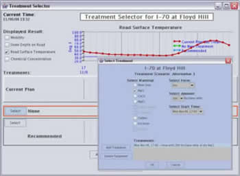
Figure 7.15. Sample image from the FHWA prototype MDSS for a plow route along Interstate 70 near Denver, CO. Winter maintenance personnel use this dialog (inset image) to enter the actual snow and ice control treatments and to explore alternative treatments. Treatment type, amount, and timing can be entered.

Vehicle data such as air and pavement temperature, ABS, vehicle stability control, and wiper settings could be also utilized by the MDSS in near real time. Air and pavement temperature data would be used to initialize the weather and road condition algorithms during each update cycle; ABS and vehicle stability control could be used within the MDSS to alert winter maintenance personnel to road segments that may need additional attention.

Vehicle probe data of air temperature coupled with wind data from RWIS or other surface observational data sources could be used to calculate local windchill temperatures, which could be use to alert maintenance staff of unsafe conditions.

7.4.2 Traffic and Incident Management

Vehicle data will provide valuable information on the state of the roadway directly to traffic managers. Traffic and congestion are sensitive to weather and road conditions. Transportation network maps that highlight wiper usage, for example, could be used by traffic and incident managers to raise their awareness that precipitation has started or that visibility is reduced due to road spray. This could provide valuable early indications of problem areas. Where applicable, traffic managers could utilize active control strategies (e.g., ramp metering to optimize flow) to mitigate problems.

Similar to wiper usage, ABS and/or vehicle stability control probe data could be used to alert traffic and incident managers of slippery road conditions. This information could be also used to notify the public via Variable Message Signs (VMS), Highway Advisory Radio (HAR) and DOT Internet sites that conditions are deteriorating.

7.4.3 Summer Maintenance

Summer maintenance activities such as pavement maintenance, pesticide spraying, road striping, and mowing are sensitive to extreme heat, high pavement temperatures, strong winds, and precipitation. Vehicle data can be used directly or integrated with other datasets as described previously to improve weather and road condition products for these end users.

Vehicle probe data of air temperature coupled with humidity data from RWIS or other surface observational data sources could be used to calculate local heat index temperatures, and to alert summer maintenance staff of unsafe conditions. Pavement temperature data measured by vehicles could be used to support striping operations. Wiper setting data could be used directly to identify road segments experiencing precipitation and to adjust mowing and pavement maintenance operations.

7.4.4 Emergency Management and Homeland Security

The current lack of a dense weather surface observation network presents significant challenges to emergency response personnel responding to hazardous chemical and/or biological releases. First responders typically obtain wind and stability information from local NWS observation sites, which can be many miles away. Wind and atmospheric stability can vary dramatically over just a few hundred feet. Local obstructions can influence wind flow and urban effects such as the heat island effect can have dramatic impacts on lower atmospheric stability, which is a critical parameter for predicting the flow and dissipation of hazardous plumes.

VII data can contribute valuable information in both rural regions and urban corridors. Dense observations of pressure and temperature from vehicles could be combined with radar and other local observations to initialize plume dispersion models. The high density of vehicle probe data in urban areas would provide critical environmental information that is generally lacking in the middle of cities. Local building effects on street level temperatures could be used to refine heat flux calculations in computational fluid dynamics models, which are now being used in research environments to study the flow in and around buildings in dense urban areas. In the next 10-20 years, these models will likely be used operationally to support emergency response operations. VII data will provide important input to these models.

Figure 7.16 illustrates the output from an urban scale plume model. Concentration levels are shown for a generic chemical being released from a single source. The general flow indicates that the hazardous plume will move toward the north through the urban corridor. Flow complexities in and around buildings are not shown in this diagram, but on the finest scales, concentration levels vary significantly from one city block to another in the center of the plume.

Vehicle data in and around the city could be used to refine stability measurements and support calculations to determine if the plume will mix with non-contaminated air through turbulence diffusion or have more laminar characteristics. Vehicle location information could be used to support evacuation decisions, as emergency response personnel would be able to view both the plume data and vehicle location data. Vehicles in harms way could be identified and notified to evacuate and be provided with guidance.

VII technologies could also be used to detect hazardous releases. Emergency personnel in Harris County, Texas instrumented a fleet of emergency vehicles (primarily police vehicles) with chemical detectors. For the year 2005 field test, they used carbon dioxide detectors. The objective of the experiment was to determine if the vehicles could be used to detect hazards and if so, could the information be communicated in near real time. The test was successful as the vehicle detectors were able to detect and transmit concentration information to the emergency management personnel. Local data were also used as input into a regional scale plume model, which was used to provide guidance to first responders. It is clear from the experiment that the operational concept was valid and this approach could be expanded nationally.

The instrumentation of fleets with supplemental weather sensors such as wind, humidity, and chemical sensors, would also provide critical input to plume models and could be used directly by emergency personnel to guide evacuation operations.

Figure 7.16. Output from an urban-scale plume dispersion model in an urban setting. Concentration levels are shown for a generic chemical released from a single source.