An Assessment of the Expected Impacts of City-Level Parking Cash-Out and Commuter Benefits OrdinancesAppendix C. Data and Analysis MethodologyThis appendix provides additional details on the data and methods applied for this study, as well as the general assumptions made during the analysis process. Data SourcesThis section describes several data sources compiled that were used in the analysis process. Table 6 shows values for each city, while the following subsections describe the data sources for each element. Locally specific data was used, wherever possible. Additionally, the team tried to identify the most recent pre-pandemic data available, if possible, such that estimates would not be skewed by potential deviations from typical behaviors or situations observed during the pandemic.21 In some cases, the team used older data sources or made assumptions based on similar cities due to data limitations. Ultimately, the selected input data reflect the best available sources—even if not ideal in all cases—at the time of analysis and were selected in consultation with the peer review group for this research. Any assumptions made for specific sources are discussed here; additional assumptions considered throughout the analysis process are presented in a later subsection. Number of Employees–CitywideThe number of employees (citywide) for each city are taken from the U.S. Census Bureau’s American Community Survey (ACS) dataset.22 For Boston/Cambridge, a sum of the employees in Boston and Cambridge was used. Number of Employees–CBDTo determine the number of employees in the CBD, the team used Demographia’s United States Central Business Districts (Downtowns) (2020) publication derived from the Census Transportation Planning Package 2012–2016. The report defines the CBD using census tracts and seeks to include the complete concentration of high-rise buildings (generally of 10 or more floors). This is a “tight” CBD definition, which is intended to include employment sites most conducive to transit commuting. The medium and lower density employment that sometimes surrounds downtown are generally excluded. Data for Cambridge is not available in the Demographia report. As such, this analysis assumes that all the employees in Cambridge work in the CBD area. Percent of Employees with Access to Free/Subsidized ParkingA variety of local data sources have been used to identify the percentage share of employees with access to free or subsidized parking at their workplace. Most reports either only reported on fully subsidized parking or provided vague information about the level of parking subsidies. Because of this, this analysis primarily considers parking cash-out policies to apply to employees with fully subsidized parking; estimates may undercount actual effects that may occur if various subsidy levels could be included in analysis.23
Percent of Employees with Access to Transit BenefitsTo estimate the percent of employees with access to transit benefits, local data for each city’s region was used where available, with many data sources overlapping those used to identify parking benefits. For the remaining cities, data from the updated 2021 National Compensation Survey by the BLS (2021 National Compensation Survey (NCS) BLS; Table 41, Quality of life benefits) was used.
Work Trip Mode Split–CitywideCitywide work trip mode splits were estimated using the U.S. Census Bureau’s ACS dataset (Table B08601 2019 5-Year Estimates by Place Geography). Work Trip Mode Split–Employees with Access to Fully Subsidized ParkingTo estimate the mode split for employees with access to fully subsidized parking, the following approaches were taken:
Average One-Way Commute Trip LengthTo estimate this measure, the team pulled commute trip length data from the 2017 National Household Travel Survey (NHTS) for all cities (except Houston, TX). Data were pulled for each city’s appropriate Metropolitan Statistical Areas, given this is the closest level of geographic granularity available in the NHTS public data. Then, the dataset was limited to home-based work trips to reflect average commute distances. Trip lengths were disaggregated by mode; NHTS mode definitions were based on the closest possible alignment with U.S. Census Bureau mode definitions in the ACS Table B08601: Means of Transportation to Work by Workplace Geography. A local data source (Central Houston 2018) was used to get estimates for Houston. CBD Parking PriceTo estimate CBD parking prices, data from Parkopedia, a parking reservation booking site and database, was used. The 2019 North American Parking Index (Parkopedia, 2020) details the 50 most expensive parking rates in North American central cities. Monthly rates were available for all cities in the current study, except for Indianapolis. The team considered other potential parking reservation websites that could provide similar data, but ultimately chose Parkopedia for the following reasons:
While Parkopedia could be used for almost all cities in this analysis, an alternative data source was needed for Indianapolis. Another parking reservation site, SpotHero, Inc., provided a data point for Indianapolis which was used to derive an estimate in line with the Parkopedia data. To estimate a monthly CBD rate for Indianapolis aligned with the Parkopedia data, a normalization factor was developed by taking the ratio of the Parkopedia parking rate to the SpotHero, Inc. parking rate for each of the remaining eight cities where data from both sources was available. An average of these normalization factors was calculated and multiplied by Indianapolis’ SpotHero, Inc. parking rate. The resulting value estimates the 2019 monthly CBD parking rate for Indianapolis. SpotHero, Inc.’s website has two alternate locations to show parking rates, both of which have different rates; as such, the above methodology was applied to both those instances. While the distinction between the two locations isn’t clear, the team hypothesized one provides historical estimates, averaged across some time, while one shows the most up-to-date parking prices. In the absence of additional information illuminating the benefit of using one datapoint over another, the study team averaged the results based on the two rates to estimate Indianapolis’s parking price. For all cities, per day parking costs were estimated from monthly parking costs by dividing the monthly cost by an estimated 19 commuting days each month. Transit FaresFor analysis purposes, the study team made no assumptions regarding the price paid for parking outside of CBDs; rather, a policy decision was made that the value of cash-out payments in non-CBD areas would be required to equal the cost of a typical monthly transit pass in the studied city. The per day cost was calculated by dividing the monthly cost by an estimated 19 commuting days each month. Transit fare data was obtained from a variety of local fare data sources:
Tax RatesThe study team compiled 2022 Federal and State income tax rates from Tax Foundation (York 2021). The average wage for an earner in each study area was determined based on a 2021 analysis by CareerBuilder®,25 and the average tax rate was computed using brackets based on that rate.
Calculating Travel ImpactsThis section describes the approach the research team took for calculating the travel impacts (i.e., the reduction in commute VMT) resulting from implementing a parking cash-out program. For some scenarios, cities in California (Los Angeles and San Diego) went through additional analytical steps. Because California has an existing cash-out requirement, the research team assumed that some share of employees at companies offering parking are already also offering cash-out. As part of its Employee Commute Survey, SANDAG (2013) reported that 5.5 percent of survey respondents indicated that they receive “cash or other incentives for not using parking” (figure 62 in that report); also, when asked if there is free parking at their work site, 90 percent out of the 99.4 percent who responded to the question, replied “yes” (figure 73 in that report). Thus, the analysis assumed that 6.1 percent of employees in California cities with free parking were also offered cash-out and that most new cash-out requirements would not impact these employees. While data comparable to that offered by this San Diego survey were not also available for Los Angeles, the two cities were considered sufficiently similar to allow the San Diego survey results to also be applied to Los Angeles. The approaches described for each scenario in this section include an explanation for adjustments, if any, made for the California cities. Note that while Washington, D.C. recently implemented a parking cash-out law (Wilson, 2022), impacts were not considered given the recency of the legislation and lag-time in observing impacts, and the pre-implementation data used in analysis. Scenario 1 (Monthly Parking Cash-Out) ApproachThe approach to analyzing an ordinance requiring employers to offer a monthly cash-out involved the following steps: Estimate the number of employees with access to parking cash-out policies. The starting point for this analysis was the total number of employees with a workplace location in each city. The analysis used available data, typically from regional travel surveys and from the U.S. Census Bureau, to estimate the share of these employees who are offered free parking (Equation 1). Equation 1. The number of employees with access to free or subsidized parking. Where:
The final employee baseline was then determined by subtracting the number of employees with access to free or subsidized parking who also have access to transit benefits. An adjustment was made later in the analysis to account for this population. Estimate the average “opportunity cost” associated with the cash-out policy. The driver response to parking cash-out offers depends on the change in driving costs. For purposes of examining travel behavior, the option to receive cash in lieu of a parking space can be viewed as an increase in the cost of driving; that is, the cash forgone is an opportunity cost to driving and parking at work. The opportunity cost is based on the market rate of parking in the city for scenarios requiring employers to offer the full cash-out value of the parking. For scenarios in which employees receive cash in lieu of parking, the cash would be considered taxable income. As such, the opportunity cost typically starts with the price of parking reduced by an average marginal tax rate (Equation 2). Equation 2. Standard opportunity cost of forgoing a parking cash out offer. Where:
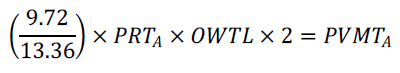
However, it is expected that rather than taking their cash-out in the form of taxable cash, employees who currently use transit or subsequently switch to transit would elect to receive—and employers would choose to offer—a tax-free transit benefit, plus any additional taxable cash to make up the difference in price between the parking cash-out value and the monthly cost of a transit pass. The research team calculated an opportunity cost for parking based on the monthly average parking rate and the monthly average transit pass cost for each city. The team assumed that commuters accepting cash-out and abandoning driving and parking would shift to alternative travel modes in proportion to their pre-existing mode shares for non-SOV travel. For the purpose of determining this opportunity cost, the cash-out value is equal to the average monthly commercial parking rate in CBDs, and outside of CBDs, the cash-out rate is assumed to be equal to the average cost of riding transit into the city. Based on this assumption, a per day rate was determined using Equation 3 through Equation 5. Equation 3. Per day monthly parking rate, weighted by CBD population. Where:
Next, the average cash-out value offered was determined as Equation 4: Equation 4. Average cash out offered, weighted by CBD population. Where, ACO = Average cash-out offered, and all other variables are as previously defined. The average benefit taken (ultimately used as the opportunity cost for analysis) is then defined as Equation 5: Equation 5. Average benefit taken (opportunity cost of driving for Scenario 1). Where, ABT = Average benefit taken, TMS = percentage of employees who do not drive alone that commute via transit, and all other variables are as previously defined. These values are displayed for the cities in this analysis in table 7.
Estimate the change in VMT with the cash-out ordinance. Based on the number of employees offered cash-out and thus experiencing the opportunity cost, the resulting reduction in trips and VMT was calculated in two different ways, described below. Version 1: Trip Reduction Impacts for Mobility Management Strategies (TRIMMS) For one approach, the research team used the TRIMMS model developed by the University of South Florida. TRIMMS is a sketch planning tool that can be used to analyze many types of strategies at a regional or sub-area scale. The tool is Microsoft® Excel-based, and preloaded with metropolitan-specific data, including employment and travel data, and travel elasticities and cross elasticities derived from national research. The user can adjust the parameter values and price elasticities. Default parameters were adjusted for starting commuter mode shares (to reflect the population receiving fully subsidized parking). TRIMMS evaluates strategies that directly affect the cost of travel, including parking pricing and public transit costs. The model uses inputs provided by the user or defaults of mode shares, average trip lengths and travel time by mode, average vehicle occupancy, parking costs, and trip costs. For this analysis, the employee populations and parking costs specific to each city were entered into TRIMMS, along with estimated initial commute mode shares for the population of employees subject to the cash-out ordinance, excluding the small portion of California employees offered cash-out because of the statewide law in advance of any city ordinances. Given that the cash-out requirement would apply only to worksites with free or subsidized parking, an estimate of mode share for employees with access to free parking was used. Additionally, the research team updated the variable identified as the auto travel elasticity with respect to parking price to -0.30 based on values identified in the literature. (Since price changes in most scenarios involve free parking as the starting condition, and an elasticity calculation is impossible if any of the values is zero, it was surmised that the input elasticity value being sought was really the price elasticity of VMT when parking pricing is included within the bundle of travel costs.) TRIMMS calculates adjusted mode shares based on the policy strategies applied. For this analysis, the final (adjusted) mode shares were pulled from the model results. By multiplying the original and final mode shares by the employee population for the city, the absolute change in commute trips was calculated (Equation 6). By applying the average trip distance by mode to the change in the number of vehicle trips, the change in VMT was calculated. Average vehicle occupancy rates were used to adjust VMT reductions from new carpool and vanpool commuters.  Equation 6. VMT reduced using TRIMMS. VMR equals EP times 2 times, begin brackets, D subscript a times the quantity (S subscript A0 minus S subscript A1), all plus D subscript R over O subscript R times the quantity (S subscript R0 minus S subscript R1), all plus D subscript V over O subscript V times the quantity (S subscript V0 minus S subscript V1), end brackets.
Where: VMR = Vehicle miles reduced Version 2: Elasticity Calculations For the second approach, the research team calculated a change in vehicle travel directly based on a travel price elasticity from the literature (i.e., without using TRIMMS). The change in vehicle travel was calculated from the percentage change in vehicle operating costs with the addition of the parking cash-out opportunity cost using an arc elasticity of -0.30 for the change in vehicle travel in relation to the parking costs as derived from the literature review (Equation 7). 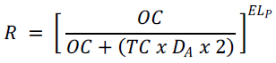 Equation 7. Percentage reduction in vehicle travel using travel elasticity. Where: R = Percentage reduction in vehicle travel The analysis assumes that employees taking the cash-out drive the same average round-trip commute distance as other drivers; thus, the percentage reduction in vehicle travel is equivalent to the percentage reduction in commute trips, or the share of drivers that accepts the cash-out offer (Equation 8). Where: VTR = Vehicle trips reduced To calculate the VMT reduction, the vehicle trips reduced were multiplied by the average driving commute distance for the area (Equation 9). Equation 9. Reduction in vehicle miles traveled for Scenario 1. Where: VMR = Vehicle miles reduced In order to compare the results to the outputs from TRIMMS, the research team used the percentage reduction in VMT from this approach to estimate a change in mode shares, assuming that the reduction in vehicle travel all came from drive-alone commute trips. The other mode shares were assumed to increase based on their relative shares from the TRIMMS results. Midpoint The TRIMMS methodology yielded an estimated 13 percent reduction in VMT in Los Angeles at worksites that would offer cash-out under Scenario 1, which is similar to the 12 percent average reduction Shoup (1997) found in his study of eight work sites, lending some support to the use of this methodology. However, the eight case studies analyzed by Shoup showed individual VMT reductions ranging from 5 percent to 24 percent, with the highest reduction levels at work sites in downtown Los Angeles (a 16 percent and 24 percent reduction, respectively). The TRIMMS approach yielded estimated impacts of cash-out for cities with high initial SOV rates, such as Indianapolis, San Diego, and Houston, that appeared quite low. By contrast, the elasticity approach made no downward adjustment in results in such cities. Specific results for affected employers (i.e., worksites offering cash-out under this scenario) from both Version 1 and Version 2 are summarized in Table 8. The elasticity-based VMT reduction figures are higher than the figures developed using TRIMMS for all cities except Boston/Cambridge and Chicago (likely due to these two cities having the lowest starting drive-alone mode share, effecting the impact of the elasticity method on drive-alone vehicle trip and VMT).
TRIMMS = Trip Reduction Impacts for Mobility Management Strategies After a discussion with the peer review group, it was decided to take a midpoint of the mode share results of the Version 1 (TRIMMS) and Version 2 (Elasticity) approaches to reflect the likely higher impacts of cash-out associated with downtown and other urban locations, but also not to overestimate the impacts. By taking a midpoint, the final mode shares lie halfway between each version’s results. The drive-alone mode shares and mid-points for each city are shown as an example in Table 9. The process for determining VMT reductions from these mode shares follows Equation 6.
TRIMMS = Trip Reduction Impacts for Mobility Management Strategies California Adjustment For Los Angeles and San Diego, the analysis described above only applied to the employee population that was not already offered parking cash-out as a result of the California mandate. Thus, trip and VMT changes in those two cities were calculated relative to travel by the baseline population of employees offered parking subsidies but not already offered cash-out. Adjustment for Employees Receiving Transit Benefits The analysis also adjusted final results to account for employees who had access to free parking, and who also had access to transit benefits. These commuters were treated differently under the assumption that, with the provision of transit benefits, their responsiveness to this policy would be expected to be somewhat muted, reflective of less change in the benefits they are offered. Making this adjustment was reliant on calculations conducted for Scenario 2 (employer-paid transit/vanpool benefit). First, VMT per employee was determined for two populations:
The percent change between the two figures—from 2) to 1)—was determined. Then, this reduction was applied to the baseline VMT for employees receiving fully subsidized parking to determine the estimated VMT reduction for this subset of employees (i.e., population 2). This reduction was added to the reduction determined in the baseline Scenario 1 analysis to get the total estimated VMT reduction. Scenario 2 (Monthly Employer-Paid Transit/Vanpool Benefit) ApproachThe research team attempted to use the TRIMMS model to estimate the impacts of an ordinance requiring employers that offer free/subsidized parking to also offer a monthly commuter benefit (e.g., transit or vanpool benefit). The results were unusually large, suggesting dramatic increases in transit mode share based on the transit price elasticities that are built into the TRIMMS model. The expectation for a monthly commuter benefit requirement under Scenario 2 is that the resulting vehicle trip reductions would be somewhat lower than the impact of offering cash-out under Scenario 1, since Scenario 1 assumes that a tax-free commuter benefit is part of the parking cash-out package, but that was not matched by the preliminary results. Consequently, the research team estimated travel impacts for Scenario 2 using the same approach as is described in the Scenario 1 analysis; however, instead of using the cash-out value as the opportunity cost, the average transit cost for each city was used instead. The baseline population for Scenario 2 was employees with access to fully subsidized parking who did not already have access to transit benefits. An output of this approach within TRIMMS was shifts to the newly subsidized modes (transit and vanpool), but also to other modes that are not subsidized (carpooling, bicycling, and walking). Initially, only shifts to the subsidized modes were accepted. Shifts to other non-SOV modes, however, show a willingness on the part of SOV drivers to entertain alternatives. Thus, for this analysis, it was then assumed that 25 percent of the employees whom TRIMMS indicated would shift to other modes based on the monetary value of the incentive would take a vanpool or transit benefit if that were the only offer instead of cash because they showed a willingness to stop driving alone. The State of New Jersey and a number of U.S. cities, including two that are being analyzed here (New York City and Washington, D.C.), have in recent years mandated that some employers make available pre-tax transit benefits to their employees. Because these requirements came into being after the period for which the data being used in this analysis were gathered, no analytical adjustments are required for these cities. California Adjustment Employees in Los Angeles and San Diego who were already offered cash-out and thus were excluded from the Scenario 1 analysis, are also excluded in this scenario; employees who were already offered cash-out are not being offered a commuter benefit in this scenario. Adjustment for Employees Receiving Transit Benefits Employees with access to fully subsidized parking who already received transit benefits were excluded in this scenario; these employees were not being offered a new commuter benefit in this scenario. Scenario 3 (Monthly Parking Cash-Out + Pre-Tax Transit Option for Employees without Subsidized Parking) ApproachUnder this scenario, in addition to the policy under Scenario 1, a pre-tax transit benefit is offered to all employees who do not have access to fully subsidized parking and who do not already receive transit benefits from their employer. The team assumed that the mode shares for the population being offered the pre-tax transit benefit were the same as the citywide shares gathered from the ACS or from regional travel surveys. The baseline population for this component of the analysis was the number of employees not receiving fully subsidized parking (or cash-out) who do not already receive transit benefits. The pre-tax transit benefit offered to employees reduces transit trip cost through tax savings or transit costs multiplied by the marginal tax rate. The research team calculated the percentage increase in transit trips by applying a transit price elasticity (reflecting the change in transit ridership in relation to a change in the price of transit) of -0.15 from the literature to the transit cost reduction. The transit trip increase was applied to the transit mode share and the use of all other modes was assumed to decline proportionally based on their original shares. Because this scenario is applied on top of the parking cash-out scenario, the trip and VMT reductions in this scenario were added to the reductions in Scenario 1 to calculate the total impact of the combined scenarios. As also noted in discussing Scenario 2, a number of jurisdictions, including two cities that are being analyzed here (New York City and Washington, DC), have in recent years mandated that some employers make available pre-tax transit benefits to their employees. Because these requirements came into being after the period for which the data being used in this analysis were gathered, no analytical adjustments are required for these cities. California Adjustment Because this scenario only applies to employees who are not offered fully subsidized parking, there is no adjustment made for Los Angeles and San Diego, as cash-out would not have been offered to any of these employees. Adjustment for Employees Receiving Transit Benefits Since the results here are added to those from Scenario 1 to understand the full impact of this policy, the adjustment made in Scenario 1 for employees eligible for cash-out who already receive transit benefits hold here. No adjustment was made for the population not receiving free parking (or cash-out) who already receive transit benefits, as a new benefit was not being offered to this population. Scenario 4 (Daily Parking Cash-Out + Pre-Tax Transit Option for Employees without Subsidized Parking) ApproachScenario 4 reflects the same policy as Scenario 3, except with daily parking cash-out. A daily cash-out option means that rather than being required to give up a parking space for a month, the employee can choose to receive cash on a daily basis whenever the employee uses an alternative to parking at work. More employees are likely to take advantage of a daily versus a monthly cash-out offer and forgo driving since they can do so on a day-by-day basis. The literature review and limited experience with more flexible parking cash-out programs support this conclusion. For the population of employees offered a daily cash-out option, the impacts of the offer are calculated from the results from Scenario 1.27 The approach is based on a study of results of the Minneapolis Innovative Parking Pricing Demonstration (Lari et al., 2014), which converted a purchased monthly parking pass to a more flexible pass that provided a small rebate on days that drivers commuted by transit instead of driving and a larger rebate when they neither drove their own car nor took transit. Since drivers purchasing the pass had an option not to purchase monthly parking at all, it was presumed that they had not accepted what was equivalent to a monthly parking cash-out offer. In this study, the most flexible Minneapolis pass option yielded a reduction in parking days of 23.8 percent. Assuming that one-third of this reduction is from telework, and that employers do not offer a cash-out on days employees do not commute at all, a daily cash-out offer was assumed to result in an additional 16 percent shift from solo driving beyond what a monthly cash-out offer would yield. This additional 16 percent reduction was applied to the results of Scenario 1 for those employees with access to the daily cash-out. The results of the adjusted Scenario 1 for daily cash-out were added to the reduction results from Scenario 3 for the population eligible for pre-tax transit benefits under this policy to estimate the total reduction under Scenario 4. California Adjustment For Los Angeles and San Diego, the scenario assumes that the employees who are already offered monthly cash-out have not yet been offered daily cash-out, and thus no adjustment was made. Adjustment for Employees Receiving Transit Benefits This adjustment was determined using the same method applied in Scenario 1. Scenario 5 (Requirement to Eliminate Subsidized Parking Benefit + Provide Universal $5 Per Day Employer-Paid Non-SOV Commute Benefit) ApproachThis scenario reflects an ordinance that requires employers that are offering their employees subsidized parking to cease offering it and for all employers to offer employer-paid non-SOV commute benefits of $5 per commute day. To calculate the trip and VMT impacts in both scenario versions, the research team recreated the approaches described in Scenarios 1, 2, and 4 although with different inputs (e.g., starting mode shares, travel costs), depending on the different employee populations being examined. Part 1: Employees at Worksites Previously Receiving Fully Subsidized Parking, Now with Unsubsidized Parking and Non-SOV Benefits For the employee population already receiving fully subsidized parking, as with Scenario 1, the research team calculated mode shares using the TRIMMS and elasticity calculation approaches and then took the midpoints between the two sets of results. Midpoint mode shares were calculated based on three cost points, modeled again as the opportunity cost of driving alone and parking:
After arriving at the midpoint mode share calculations for each of the three cost points above, the final mode shares for this population were determined by:
Because this scenario assumes a daily non-SOV benefit and daily parking costs, an additional 16 percent mode shift away from driving alone was applied as in Scenario 4. An adjustment for employees receiving transit benefits was made to the final VMT reduction as in Scenario 1, which also relies on data from Scenario 2. Part 2: California Adjustment This scenario assumes the cash-out ordinances in Los Angeles and San Diego would hold. As such, VMT reductions were estimated separately for this population. The analysis process followed that outlined in Part 1, except with slightly different cost points:
Again, because this scenario assumes a daily non-SOV benefit and daily parking costs, an additional 16 percent mode shift away from driving alone was applied as in Scenario 4. An adjustment for employees receiving transit benefits was made to the final VMT reduction as in Scenario 1, which also relies on data from Scenario 2. However, a separate run of Scenario 2 was estimated specifically for this population to apply for this adjustment, using the mode shares estimated from the first cost-point above as the starting mode shares for the population already receiving cash-out in the California cities. Part 3: Employees Who Were Not Receiving Fully Subsidized Parking and Now Receive a Non-SOV Benefit VMT reduction for this population was again determined as in Part 1, but only with the following two cost points since this population experiences no impacts to parking costs:
Final mode shares were determined as in Part 1, except the drive alone mode share was taken from the baseline mode share for employees not receiving fully subsidized parking and adjusted using the same method in Part 1. Baseline mode shares for employees not receiving fully subsidized parking were estimated by subtracting the number of employees receiving fully subsidized parking from the number of employees citywide commuting by each mode for each city, and then calculating the total share of that population taking each mode. Again, because this scenario assumes a daily non-SOV benefit and daily parking costs, an additional 16 percent mode shift away from driving alone was applied as in Scenario 4. An adjustment for employees receiving transit benefits was made to the final VMT reduction as in Scenario 1, which also relies on data from Scenario 2. However, a separate run of Scenario 2 was estimated specifically for this population to apply for this adjustment, starting with the mode share for employees not receiving fully subsidized parking. Scenario 1A (Monthly Parking Cash-Out for Employees Working for Employers with 20 or More Employees) ApproachThis scenario adjusts the results of Scenario 1 to account only for employees working for firms with 20 or more employees; this employer size exclusion follows that put forward by Washington, D.C.’s, parking cash-out law. Additional information and results on this analysis are provided in Appendix D. Additional Results. There are two overall things required to estimate the impact of the scenario extension to exempt small-employers. The first is to understand the number of employees in the cities working for exempt employers. The second, since the impact of the policies vary based on “starting” commute benefits offers, is understanding the degree to which small-employer benefits offerings differ from other employers. To estimate the number of employees working for firms with 20 or more employees who would be subject to this policy, data from the Seattle Employer Transportation Benefits Survey (Commute Seattle, 2016) was used to determine the differences in benefits offerings by employer size. This was the only data source that could be found, after an exhaustive search, that differentiates commuter benefits by employer size at a comparable scale (i.e., across an entire jurisdiction) that enabled the team to adjust the data appropriately. The percent of employees receiving free parking and subsidized transit benefits overall were calculated. Then, these percentages were calculated for employees working for firms with 20–100 employees, followed by for employers with more than 100 employees.28 Differentiation between these categories were made given that employers with more than 500 employees were not surveyed. As such, the team assumed that the largest employers (500+ employees) would match the benefits offerings patterns of large employers (100–499 employees). The benefits offerings for the mid- and large-size employers were compared to the overall rate to develop a scaling factor for the citywide rates used in this analysis. If the mid- or large-employer rate was higher than the citywide rate, the gap between both rates and 100 percent was determined. Then, the difference was divided by the gap between the citywide rate and 100 percent to determine the scaling factor. This factor would be used to “scale up” the commute benefits offerings from the employers not exempt from the policy. If the mid- or large-employer rate was lower than the citywide rate, the gap between both rates and 0 percent was determined (this is equal to the standing percentages). Then, the difference was divided by the citywide rate to determine the scaling factor to “scale down” the commute benefits offerings. This method to derive the scaling factors, and then to appropriately scale the citywide estimates, is shown in Equations 10 and 11. Example calculations for parking benefits in Seattle are shown in Equations 12 and 13 using the data in Table 10.
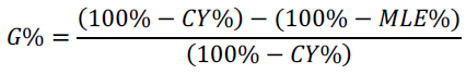 Equation 10. Scaling factor equation when the mid or large size employer offering is greater than the citywide offering. Where:
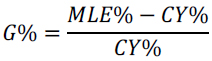 Equation 11. Scaling factor equation when the mid or large size employer offering is less than the citywide offering. Where:
Using Equation 10 and Equation 11, the team arrived at the scaling factors presented in Table 11. An example use of these factors to scale the free parking offering in Houston, TX (41 percent) is shown in Equation 12 and Equation 13.
Equation 12. Sample calculation. Estimating the percentage of Employees Working for Firms with 20–99 Employees Receiving Free Parking Benefits in Houston, TX [this equation format used to apply an increase, or closing the gap toward 100 percent] Equation 13. Sample calculation. Estimating the percentage of Employees Working for Firms with 100+ Employees Receiving Free Parking Benefits in Houston, TX [this equation format used to apply a decrease, or closing the gap toward 0 percent] Citywide free parking and transit benefits figures were scaled for all cities. The new baseline population for Scenario 1A was then determined using these new figures, along with data using the Census Statistics of U.S. Businesses (SUSB) Annual Data Tables by Establishment Industry (U.S. Census Bureau 2018). These tables provided estimates of the percentage of employees working for firms between 20–99 employees, and then for firms with 100 or more employees. The results from Scenario 1 were then scaled appropriately based on the difference in the number of employees being served by the policy, and the new citywide commute VMT reductions were calculated. Scenario 3A (Monthly Parking Cash-Out + Pre-Tax Transit Option for Employees without Subsidized Parking for Employees Working for Employers with 20 or More Employees) ApproachRecall that, to determine the effects of Scenario 3, the impact of the pre-tax transit option for employees without subsidized parking was added to the results of Scenario 1 to determine the overall effect of this policy. Here, the new baseline number of employees eligible for pre-tax transit benefits was determined using the same scaling factors and process as in Scenario 1A to scale the initial results from Scenario 3. Then, these results were added to the reductions calculated in Scenario 1A to determine the overall impact of this scenario. Calculating Resulting Congestion, Environmental, and Safety ImpactsTo calculate the impact of parking cash-out policies on driving-related externalities and costs, the research team first determined reductions to actual commute VMT based on expectations in telework after the COVID-19 pandemic, and then applied per-mile factors to the estimated reductions to arrive at measures for congestion and environmental impacts. Accounting for TeleworkThe research team investigated several sources on expectations for telework after the COVID-19 pandemic. Mokhtarian, Wang, and Kim (2022), through a series of surveys, estimated post-pandemic telework occasions to be between 1.4x to 3.2x pre-pandemic rates, with the “most likely” scenario being around 2x pre-pandemic rates. Based on these estimates, the team scaled down the baseline number of commuters identified based on pre-pandemic data (along with baseline commute VMT) to account for increased telework. Total percentage VMT reductions determined through each scenario were then applied to this reduced baseline to determine the raw VMT reduction under each scenario. Raw VMT reductions are reported for the full range provided by Mokhtarian, Wang, and Kim (2022). Congestion, environmental, and safety impacts were then determined based on the most likely scenario (2x pre-pandemic rates). EmissionsTo calculate criteria pollutant and GHG emission impacts of the policy scenarios, regional average per-mile emission factors for CO2e, oxides of nitrogen (NOx), and fine particulate matter (PM-2.5) were pulled from TRIMMS; these emissions factors are from the EPA’s Motor Vehicle Emission Simulator model (MOVES 2010a)29. The per-mile emission rates were multiplied by the VMT reductions to calculate the change in running emissions (Equation 14): Equation 14. Total emissions reduced for pollutant p. Where:
CongestionCongestion benefits are highly dependent upon local factors and require detailed modeling for accuracy. The latest version of the TRIMMS model included new data from which congestion could be estimated. Namely, data in TRIMMS lent itself to three potential congestion estimates;30 the research team estimated results for each. In estimating congestion aligned with each method, the research team estimated that 90 percent of commute VMT occurs during peak hours. Before applying congestion data from TRIMMS, the research team took the following steps:
Next, the team tested results from each potential methodological approach available given data provided in TRIMMS: Method 1: Using Average Added Delay TRIMMS provides a regional-specific measure of average added delay (minutes per VMT). To estimate impacts of the scenarios on peak-hour congestion using this method, peak baseline minutes of delay and the percent change in congestion based on that delay for each scenario were estimated for each city using the derived all peak VMT value and average added delay from TRIMMS (Equation 16 a-c).  Equation 16 a-c. Percent change in congestion (vehicle minutes of delay), Method 1. Where:
Method 2: Using Elasticity TRIMMSv4.0 calculated elasticities reflecting the percentage change in delay relative to a 1 percent change in VMT using a panel regression (accounting for total delay, area VMT, land area density, real per capita gross domestic product, and year fixed-effects to control for variation over time). The derived elasticities are specific to urban area size, as presented in Table 13. All cities in this study fall into the “Very Large” urban area size category (>3M people), except for Indianapolis, which is classified as a “Large” area (1–3M people).
To estimate the impact of each scenario on delay using this method, the percent change in all peak VMT as a result of each policy scenario was multiplied by the appropriate elasticity for each city (equation 17). Equation 17. Percent change in congestion (vehicle minutes of delay), Method 2. Where:
Method 3: Marginal Added Delay The third method applied to estimate congestion impacts of the scenarios combines approaches from the previously described two methods. The method starts with baseline delay, BPD, as measured in Equation 16. Unlike Method 1, Method 3 does not assume that baseline delay factor holds for changes in VMT introduced to the system. Instead, Method 3 estimates marginal added delay, in minutes, for the additional VMT change, as suggested by TRIMMS and in Equation 18. 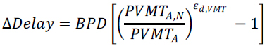 Equation 18. Marginal added delay. Where:
Then, the percent change in delay is calculated as shown below, where all variables are as previously defined (Equation 19): 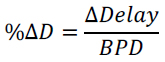 Equation 19. Percent change in congestion (vehicle minutes of delay), Method 3. Ultimately, as briefly touched upon in Chapter 3. City And Scenario Selection, the research team selected Method 3 given its use of both city-specific baseline delay data and the area-size-specific elasticity value that reflected a more sophisticated (i.e., non-linear) relationship between delay and VMT. Method 3 combined the individual advantages offered by Method 1 and Method 2. SafetyAfter consulting the peer review group convened for this research, the team believed it was reasonable to assume reductions in crashes would scale linearly with reductions in VMT for this sketch-level analysis. Deviations from this standard trend during the COVID-19 pandemic might be attributed to higher levels of speeding during this time (Litman, 2022b), which is expected to dissipate as the causes start to recede (e.g., near-empty roadways and pandemic-inspired antisocial behavior). Real numbers of avoided crashes were estimated using estimated VMT reductions (accounting for telework expectations) and the regionally-specific crash rates (crashes on the KABCO Injury Classification Scale33 per million VMT) provided in TRIMMS. 21 Note that post-pandemic expectations are accounted for later in this analysis through telework expectations. [ Return to Note 21 ] 22 See the data from ACS Table B08601 2019 5-Year Estimates by Workplace Geography here: https://data.census.gov/table?q=B08601&tid=ACSDT5Y2019.B08601 [ Return to Note 22 ] 23 See Appendix D. Additional Results for additional discussion on this matter. [ Return to Note 23 ] 24 Houston’s survey included two different response options to indicate the offering of a parking subsidy. One response option clearly indicated that the parking was free while the second was more ambiguous. Given Houston shares many characteristics of other lower-density cities that FHWA analyzed with relatively high rates of free and subsidized parking, FHWA considered adding the positive responses (for a sum of 41 percent) from the survey together to be reasonable. [ Return to Note 24 ] 25 See https://www.careerbuilder.com/advice/average-salary-by-city. [ Return to Note 25 ] 26 Equivalent to the percentage reduction in commuter trips. [ Return to Note 26 ] 27 Note that Scenario 1 calculations are based on monthly market parking rates. While daily parking costs more in the marketplace than pro-rated monthly parking, the daily cash-out rate, as envisioned and modeled, was based on the pro-rated monthly cash-out costs. [ Return to Note 27 ] 28 These cutoffs were used so they could be aligned with data on the percentage of employees working for firms of different sizes from the Census 2018 SUSB Annual Data Tables by Establishment Industry. [ Return to Note 28 ] 29 The team explored opportunities to update emissions rates based on newer data sources; however, temporal and spatial data limitations led the team to conclude that the rates developed in TRIMMS were the most appropriate to use, save from re-running EPA’s latest version of MOVES for the nine cities analyzed. [ Return to Note 29 ] 30 Additional information about the measures used can be found in the TRIMMS 4.0 documentation, accessed at https://mobilitylab.org/calculators/download-trimms-4-0/ [ Return to Note 30 ] 31 Values obtained from TRIMMS v4.0 tool. Note that TRIMMS reports values at the metropolitan-area level. As such, some values may be less accurate for cities, a caveat to the congestion estimation approach. For example, one might expect New York City’s average delay to be similar to that in other large, dense cities. In contrast, the value presented in Table 14 is lower in New York’s metro region than other metro regions, likely because the concentrated added delay factor one might observe within the city is diluted by lower added delay factors across the metropolitan region. [ Return to Note 31 ] 32 Values obtained from TRIMMS v4.0 documentation. Although the cities in this study fall only into the “Large” and “Very Large” size categories, it is worth noting that the elasticity for “Small” urban areas may be greater than that for the largest urban areas given network capacity constraints. That is, with smaller networks, it may not take much in terms of additional vehicles added to the system before congestion impacts become very substantial in such areas. [ Return to Note 32 ] 33 KABCO Injury Classification Scale: K = Fatality, a victim was killed; A = Incapacitating injury, a victim suffered incapacitating injuries that require hospitalization and/or transport for medical care, such as broken bones, amputation; B = Non-incapacitating injury, injuries to victims were evident to officers at the scene, but they were non-disabling lacerations, scrapes, or minor bruises; C = Possible injury, a victim suffered possible injuries; O = Property-damage only, there were no apparent injuries involved in the crash. [ Return to Note 33 ] | ||||||||||||||||||||||||||||||||||||||||||||||||||||||||||||||||||||||||||||||||||||||||||||||||||||||||||||||||||||||||||||||||||||||||||||||||||||||||||||||||||||||||||||||||||||||||||||||||||||||||||||||||||||||||||||||||||||||||||||||||||||||||||||||||||||||||||||||||||||||||||||||||||||||||||||||||||||||||||||||||||||||||||||||||||||||||||||||||||||||
|
United States Department of Transportation - Federal Highway Administration |
||